Demand Estimation Chapter 5
Demand Estimation Chapter 5. What will happen to quantity demanded, total revenue and profit if we increase prices? What will happen to demand if consumer incomes increase or decrease due to an economic expansion or contraction? What affect will a tuition increase have on Marquette’s revenue?.

Demand Estimation Chapter 5
E N D
Presentation Transcript
Demand Estimation Chapter 5 • What will happen to quantity demanded, total revenue and profit if we increase prices? • What will happen to demand if consumer incomes increase or decrease due to an economic expansion or contraction? • What affect will a tuition increase have on Marquette’s revenue?
Practical Example: Port Authority Transit Case • How will the fare price increase affect demand and overall revenues? • What other factors, besides fares, affect demand?
Demand Estimation Using Market Research Techniques • How do we estimate the Demand Function? • Econometric Techniques (Your Project) • Non-econometric Techniques • Look first at Non-econometric Approaches • What are these?
Question customers to estimate demand “How many bags of chips would you buy if the price was $2.29/bag?” “How many cases of beer would you buy if the price of beer was $11.99/case?” Compare different individuals’ responses WES example Advantages: Flexible Relatively inexpensive to conduct Disadvantages Many potential biases Strategic Information Hypothetical Interviewer Consumer Surveys: Just Ask Them
Market Experiments • Firms vary prices and/or advertising and compare consumer behavior • Over time (e.g., before and after rebate offer) • Over space (e.g., compare Milwaukee and Minneapolis consumption when prices are varied between two regions) • Potential Problems • Control of other factors not guaranteed. • “Playing” with market prices may be risky. • Expensive
Simulated market setting in which consumers are given income to spend on a variety of goods The experimenters control income, prices, advertising, packaging, etc. Advantages Flexibility Disadvantages Selectivity bias Very expensive Consumer Clinics and Focus Groups
Econometrics • “Economic Measurement” • Collection of statistical techniques available for testing economic theories by empirically measuring relationships among economic variables. • Quantify economic reality – bridge the gap between abstract theory and real world human activity.
Practical Example • How does the state of Wisconsin set a budget? • What is the process?
The Econometric Modeling Process • Specification of the theoretical model • Identification of the variables • Collection of the data • Estimation of the parameters of the model and their interpretation • Development of forecasts (estimates) based on the model
Numbers Instead of Symbols! • Normal model of consumer demand • Q = f(P, Ps, Id) • Q = quantity demanded of good, P = good price, Ps = price of substitute good, Id = disposable income • Econometrics allows us to estimate the relationship between Q and P, Ps and Id based on past data for these variables
Q = 31.5 – 0.73P + 0.11Ps + 0.23Yd • Instead of just expecting Q to “increase” if there is an increase in Id – we estimate that Q will increase by 0.23 units per 1 dollar of increased disposable income • 0.23 is called an estimated regression coefficient • The ability to estimate these coefficients is what makes econometrics useful
Regression Analysis • One econometric approach • Most popular among economists, business analysis and social sciences • Allows quantitative estimates of economic relationships that previously had been completely theoretical • Answer “what if” questions
Regression Analysis Continued • Regression analysis is a statistical technique that attempts to “explain” movements in one variable, the dependent variable, as a function of movements in a set of other variables, called the independent (or explanatory) variables, through the quantification of a single equation. • Q = f(P, Ps, Yd) • Q = dependent variable • P, Ps , Yd = independent variables • Deals with the frequent questions of cause and effect in business
What is Regression Really Doing? • Regression is the fitting of curves to data. P More later! Q
Gathering Data • Once the model is specified, we must collect data. • Time-series data • e.g., sales for my company over time. • What most of you will be using in your projects. • Cross-sectional data • e.g., sales of 10 companies in the food processing industry at one point in time.
Garbage In, Garbage Out • Your empirical estimates will be only as reliable as your data. • Look at the two quotes from Stamp and Valavanis that follow. • You will want to take particular care in developing your databases.
Sir Josiah Stamp“Some Economic Factors in Modern Life” • The government are very keen on amassing statistics. They collect them, add them, raise them to the n’th power, take the cube root and prepare wonderful diagrams. But you must never forget that every one of those figures comes in the first instance from the village watchman, who just puts down what he damn well pleases. • Moral: Know where your data comes from!
Valavanis • “Econometric theory is like an exquisitely balanced French recipe, spelling out precisely with how many turns to mix the sauce, how many carats of spice to add, and for how many milliseconds to bake the mixture at exactly 474 degrees of temperature.”
Valavanis - continued • “But when the statistical cook turns to raw materials, he finds that hearts of cactus fruit are unavailable, so he substitutes chunks of cantaloupe; where the recipe calls for vermicelli he uses shredded wheat; and he substitutes green garment dye for curry, ping-pong balls for turtle’s eggs, and, for Chaligougnac vintage 1883, a can of turpentine.” • Moral: Be careful in your choice of proxy variables
Economic Data • You are in the process of gathering economic data. • Some will come from your firm. • Some may come from trade publications. • Some will come from the government. • Must be of the same time scale (monthly, quarterly, yearly, etc.)
Always be Skeptical • Always approach your data with a critical eye. • Remember the quotes • Just because something appears in a table somewhere, does not mean it is necessarily correct. • Government data revisions. • Does your data pass the “smell test”?
How to Begin the Data Exercise • First question you should ask yourself is: • “If money were no object, what would be the perfect data for my demand model?” • From that basis, you can then start finding what actual data you can get your hands on. • There will be compromises that you have to make. These are called proxy variables! • Remember the Valavanis quote.
How to Choose a Good Proxy • Proxy variables should be variables whose movements closely mirror the desired variable for which you do not have a measure. • For example: Tastes of consumers are difficult to measure. • May use a time trend variable if you suspect these are changing over time. • May include demographic characteristics of the population.
Dummy Variables • Binary Variable • Take on a “1” or a “0” • Example: Trying to model salaries • 1 if you have a college degree, 0 if you don’t • Example: Model effect of Harley-Davidson reunion years on demand • 1 for reunion years, 0 otherwise
Back to Regression Analysis • Theoretical Model: Y = 0 + 1X + • Y is dependent variable • X is independent variable • Linear Equation (no powers greater than 1) • ’s are coefficients – determine coordinates of the straight line at any point • 0 is the constant term – value of Y when X is 0 (more on this later - no economic meaning but required) • 1 is the slope term – amount Y will change when X increases by one unit (can be 2 … n) holds all other ’s constant (except those not in model!) • More about , the error term, later
Graphical Representation of Regression Coefficients Regression Line Y Y = 0 + 1X Y 1 X 0 X
The Error Term • Y = 0 + 1X + • is purely theoretical • Stochastic Error Term Needed Because: • Minor influences on Y are omitted from equation (data not available) • Impossible not to have some measurement error in one of the equation’s variables • Different functional form (not linear) • Pure randomness of variation (remember human behavior!)
Example of Error • Trying to estimate demand for SUV’s • Demand may fall because of uncertainty about the economy (what data do we use for uncertainty?) • Other independent variables may be omitted • Demand function may be non-linear • Demand for SUV’s is determined by human behavior – some purely random variation • All end up in error term
The Estimated Regression Equation • Theoretical Regression Equation: Y = 0 + 1X + • Estimated Regression Equation: Y^ = 103.40 + 6.38X + e • Observed, real word X and Y values are used to calculate coefficient estimates 103.40 and 6.38 • Estimates are used to determine Y-hat, the fitted value of Y • “Plug-in” X and get estimate of Y
Differences Between Theoretical and Estimated Regression Equations • 0, 1 replaced with estimates 0^, 1^ (103.40 and 6.38) • Can’t observe true coefficients, we make estimates • Best guesses given data for X and Y • Y^ is estimated value of Y – calculated from the regression equation (line through Y data) • Residual e = Y – Y^ • Residual is difference between Y (data) and Y^ (estimated Y with regression) • Theoretical model has error, estimated model has residual
A Simple Regression Example in Eviews • Demand for Ford Taurus
Ordinary Least Squares Regression • OLS Regression • Most Common • Easy to use • Estimates have useful characteristics
How Does Ordinary Least Squares Regression Work? • We attempt to find the curve that best fits the data among all possibilities • While there are a number of ways of doing this, OLS minimizes the sum of the squared residuals
Finding Best Fitting Line using Ordinary Least Squares Actual data points are dependent variable (Y’s) Y = 0 + 1X + Y^ = 0^ + 1^X + e “hat” is sample estimate of true value OLS minimizes: e 2 e = (Y – Y^) OLS minimizes (Y-Y^)2 P _ P _ Q Q Best possible linear line through data
True vs. Estimated Regression Line • No one knows the parameters of the true regression line: Yt = + Xt + t (theoretical) • We must come up with estimates. Y^t = ^ + 1^Xt + et (estimated)
So how does OLS work? • OLS selects the estimates of 0 and 1 that minimize the squared residuals • Minimize difference between Y and Y^ • Statistical Software • Complex math behind the scenes
OLS Regression Coefficient Interpretation • Regression coefficients (’s) indicate the change in the dependent variable associated with a one-unit increase in the independent variable in question holding constant the other independent variables in the equations (but not those not in the equation) • A controlled economic experiment?
Another Example • The demand for beef • B = 0 + 1P + 2Yd • B = per capita consumption of beef per year • Yd = per capita disposable income per year • P = price of beef (cents/pound) • Estimate this using Eviews
Overall Fit of the Model • Need a way to evaluate model • Compare one model with another • Compare one functional form with another • Compare combinations of independent variables • Use coefficient of determination r2
r2 – The Coefficient of Determination • Reported by Eviews every time you run a regression • Between 0 and 1 • The larger the better • Close to one shows an excellent fit • Near zero shows failure of estimated regression to explain variance in Y • Relative term • r2 = .85 says that 85% of the variation in the dependent variable is explained by the independent variables
Graphical r2 • r2 = 0 • r2 = .95 • r2 = 1
The Adjusted r2 • Problem with r2: Adding another independent variable never decreases r2 • Even a nonsensical variable • Need to account for a decrease in “degrees of freedom” • Degrees of freedom = data observations – coefficients estimated • Example: 100 years of data, 3 variables estimated (including constant) • DF = 97
Adjusted r2 • Slightly negative to 1 • Accounts for degrees of freedom • Better estimate of fit • Don’t rely on any one statistic • Common sense and theory more important • Same interpretation as r2 • Use adjusted r2 from now on!
The Classical Linear Regression (CLR) Model • These are some basic assumptions which when met, make the Ordinary Least Squares procedure the “Best Linear Unbiased Estimator” (aka BLUE). • When one or more of these assumptions is violated, it is sometimes necessary to make adjustments to our model.
Assumptions(Yt=X1t+ X2t+...+t) • Linearity in coefficients and error term • has zero population mean • All independent variables are independent of • Error term observations are uncorrelated with each other (no serial correlation) • has constant variance (no heteroskedasticity) • No independent variables are perfectly correlated (multicollinearity) Will come back to some of these when we test our models
1st Assumption: Linearity • We assume that the model is linear (additive) in the coefficients and in the error term, and specification is correct. • e.g., Yt=X1+ X2+is is linear in both, whereas Yt=X1+ X2+is not. • Some nonlinear models can be transformed into linear models. • e.g., Yt=X1X2 • We showed this can be transformed using logs to: lnYt=lnlnX1+ lnX2+ ln
Hypothesis Testing • In statistics we cannot “prove” a theory is correct • Can “reject” a hypothesis with a certain degree of confidence
Common Hypothesis Test • H0: = 0 – Null Hypothesis • HA: 0 – Alternative Hypothesis • Test whether or not the coefficient is statistically significantly different from zero • Does the coefficient affect demand? • Two-tailed test
Does Rejecting the Null Hypothesis Guarantee that the Theory is Correct? • NO! It is possible that we are committing what is known as a Type I error. • A Type I error is rejecting that Null hypothesis when it is in fact correct. • Likewise, we may also commit a Type II error • A Type II error is failing to reject the Null hypothesis when the alternative hypothesis is correct.
Type I and Type II Error Example • Presumption of innocence until proven guilty • H0: The defendant is innocent • HA: The defendant is guilty • Type I error: sending an innocent defendant to jail • Type II error: freeing a guilty defendant