Mastering Demand Estimation and Forecasting in Business
Explore regression analysis, forecasting techniques, and challenges in demand estimation. Learn to interpret results and ensure statistical significance in forecasting methods. Understand data collection sources and the importance of accurate data for business analysis.

Mastering Demand Estimation and Forecasting in Business
E N D
Presentation Transcript
Chapter 5 Demand Estimation and Forecasting
Chapter Outline • Regression analysis • Limitation of regression analysis • The importance of business forecasting • Prerequisites of a good forecast • Forecasting techniques
Learning Objectives • Understand the importance of forecasting in business • Know how to specify and interpret a regression model • Describe the major forecasting techniques used in business and their limitations • Explain basic smoothing methods of forecasting, such as the moving average and exponential smoothing
Data Collection • Statistical analyses are only as good as the accuracy and appropriateness of the sample of information that is used. • Several sources of data for business analysis: • buy from data providers (e.g. ACNielsen, IRI) • perform a consumer survey • focus groups • technology: point-of-sale data sources
Regression Analysis • Regression analysis: a procedure commonly used by economists to estimate consumer demand with available data Two types of regression: • cross-sectional: analyze several variables for a single period of time • time series data: analyze a single variable over multiple periods of time
Regression Analysis • Regression equation: linear, additive eg: Y = a + b1X1 + b2X2 + b3X3 + b4X4 Y: dependent variable a: constant value, y-intercept Xn: independent variables, used to explain Y bn: regression coefficients (measure impact of independent variables)
Regression Analysis • Interpreting the regression results: Coefficients: • negative coefficient shows that as the independent variable (Xn) changes, the variable (Y) changes in the opposite direction • positive coefficient shows that as the independent variable (Xn) changes, the dependent variable (Y) changes in the same direction • The regression coefficients are used to compute the elasticity for each variable
Regression Analysis • Statistical evaluation of regression results: • t-test: test of statistical significance of each estimated coefficient (whether the coefficient is significantly different from zero) b = estimated coefficient Seb = standard error of estimated coefficient
Regression Analysis • Statistical evaluation of regression results: • ‘rule of 2’: if absolute value of t is greater than 2, estimated coefficient is significant at the 5% level (for large samples-for small samples, need to use a t table) • if coefficient passes t-test, the variable has a significant impact on demand
Regression Analysis • Statistical evaluation of regression results • R2 (coefficient of determination): percentage of variation in the variable (Y) accounted for by variation in all explanatory variables (Xn) R2value ranges from 0.0 to 1.0 The closer to 1.0, the greater the explanatory power of the regression.
Regression Analysis • Statistical evaluation of regression results • F-test: measures statistical significance of the entire regression as a whole (not each coefficient)
Regression Analysis • Steps for analyzing regression results • check coefficient signs and magnitudes • compute elasticity coefficient • determine statistical significance
Regression Analysis • Textbook example: Management lessons from estimating demand for pizza • demand for pizza affected by • price of pizza • price of complement (soda) • managers can expect price decreases to lead to lower revenue • tuition and location are not significant
Regression Analysis • Challenges • Identification • Multicollinearity • Autocorrelation
Regression Analysis • Challenge 1: Identification problem: • The estimation of demand may produce biased results due to simultaneous shifting of supply and demand curves. • Solution: use of advanced correction techniques, such as two-stage least squares and indirect least squares may compensate for the bias
Regression Analysis • Challenge 2: Multicollinearity problem • Two or more independent variables are highly correlated, thus it is difficult to separate the effect each has on the dependent variable. • Solution: a standard remedy is to drop one of the closely related independent variables from the regression
Regression Analysis • Challenge 3: Autocorrelation problem • Also known as serial correlation, occurs when the dependent variable relates to the Y variable according to a certain pattern • Note: possible causes include omitted variables, or non-linearity; Durbin-Watson statistic is used to identify autocorrelation • Solution: to correct autocorrelation consider transforming the data into a different order of magnitude or introducing leading or lagging data
Forecasting • “Forecasting is very difficult, especially into the future.” • Common subjects of business forecasts: • gross domestic product (GDP) • components of GDP • examples: consumption expenditure, producer durable equipment expenditure, residential construction • industry forecasts • example: sales of products across an industry • sales of a specific product
Forecasting • A good forecast should: • be consistent with other parts of the business • be based on knowledge of the relevant past • consider the economic and political environment as well as changes • be timely
Forecasting Techniques • Factors in choosing the right forecasting technique: • item to be forecast • interaction of the situation with the forecasting methodology--the value and costs • amount of historical data available • time allowed to prepare forecast
Forecasting Techniques • Six forecasting techniques • expert opinion • opinion polls and market research • surveys of spending plans • economic indicators • projections • econometric models
Forecasting Techniques • Approaches to forecasting • qualitative forecasting is based on judgments expressed by individuals or group • quantitative forecasting utilizes significant amounts of data and equations
Forecasting Techniques • Approaches to quantitative forecasting: • naïve forecasting projects past data without explaining future trends • causal (or explanatory) forecasting attempts to explain the functional relationships between the dependent variable and the independent variables
Forecasting Techniques • Expert opinion techniques • Jury of executive opinion: forecasts generated by a group of corporate executives assembled together
Forecasting Techniques • Expert opinion techniques • The Delphi method: a form of expert opinion forecasting that uses a series of questions and answers to obtain a consensus forecast, where experts do not meet
Forecasting Techniques • Opinion polls: sample populations are surveyed to determine consumption trends • may identify changes in trends • choice of sample is important • questions must be simple and clear
Forecasting Techniques • Market research: is closely related to opinion polling and will indicate not only why the consumer is (or is not) buying, but also • who the consumer is • how he or she is using the product • characteristics the consumer thinks are most important in the purchasing decision
Forecasting Techniques • Surveys of spending plans: yields information about ‘macro-type’ data relating to the economy, especially: • consumer intentions • examples: Survey of Consumers (University of Michigan), Consumer Confidence Survey (Conference Board) • inventories and sales expectations
Forecasting Techniques • Economic indicators: a barometric method of forecasting designed to alert business to changes in conditions • leading, coincident, and lagging indicators • composite index: one indicator alone may not be very reliable, but a mix of leading indicators may be effective
Forecasting Techniques • Leading indicators predict future economic activity • average hours, manufacturing • initial claims for unemployment insurance • manufacturers’ new orders for consumer goods and materials • vendor performance, slower deliveries diffusion index • manufacturers’ new orders, nondefense capital goods
Forecasting Techniques • Additional leading indicators to predict future economic activity • building permits, new private housing units • stock prices, 500 common stocks • money supply, M2 • interest rate spread, 10-year Treasury bonds minus federal funds • index of consumer expectations
Forecasting Techniques • Coincident indicators identify trends in current economic activity • employees on nonagricultural payrolls • personal income less transfer payments • industrial production • manufacturing and trade sales
Forecasting Techniques • Lagging indicators confirm swings in past economic activity • average duration of unemployment, weeks • ratio, manufacturing and trade inventories to sales • change in labor cost per unit of output, manufacturing (%)
Forecasting Techniques • Additional lagging indicators confirm swings in past economic activity • average prime rate charged by banks • commercial and industrial loans outstanding • ratio, consumer installment credit outstanding to personal income • change in consumer price index for services
Forecasting Techniques • Economic indicators: drawbacks • leading indicator index has forecast a recession when none ensued • a change in the index does not indicate the precise size of the decline or increase • the data are subject to revision in the ensuing months
Forecasting Techniques • Trend projections: a form of naïve forecasting that projects trends from past data without taking into consideration reasons for the change • compound growth rate • visual time series projections • least squares time series projection
Forecasting Techniques • Compound growth rate: forecasting by projecting the average growth rate of the past into the future • provides a relatively simple and timely forecast • appropriate when the variable to be predicted increases at a constant percentage
Forecasting Techniques • General compound growth rate formula: E/B = (1+i)n E = final value n = years in the series B = beginning value i = constant growth rate
Forecasting Techniques • Visual time series projections: plotting observations on a graph and viewing the shape of the data and any trends
Forecasting Techniques • An Example in Which the Constant Compound Growth Rate Approach Would Be Misleading
Forecasting Techniques • Time series analysis: a naïve method of forecasting from past data by using least squares statistical methods to identify trends, cycles, seasonality, and irregular movements
Forecasting Techniques • Time series analysis: • easy to calculate • does not require much judgment or analytical skill • describes the best possible fit for past data • usually reasonably reliable in the short run
Forecasting Techniques • Time series data can be represented as: Yt = f(Tt, Ct, St, Rt) Yt = actual value of the data at time t Tt = trend component at t Ct = cyclical component at t St = seasonal component at t Rt = random component at t
Forecasting Techniques • Time series components: seasonality • need to identify and remove seasonal factors, using moving averages to isolate those factors • remove seasonality by dividing data by seasonal factor
Forecasting Techniques • Time series components: trend • to remove trend line, use least squares method • possible best-fit line styles: straight line: Y = a + b(t) exponential line: Y = abt quadratic line: Y = a + b(t) + c(t)2 • choose one with best R2
Forecasting Techniques • Time series components: cyclical, random • isolate cyclical components by smoothing with a moving average • random factors cannot be predicted and should be ignored
Forecasting Techniques • Smoothing techniques • Moving average • The larger the number of observations in the average, the greater the smoothing effect. • Exponential smoothing • Allows for the decreasing importance of information in the more distant past.
Forecasting Techniques • Moving average: average of actual past results used to forecast one period ahead Et+1 = (Xt + Xt-1 + … + Xt-N+1)/N Et+1 = forecast for next period Xt, Xt-1 = actual values at their respective times N = number of observations included in average
Forecasting Techniques • Exponential smoothing: allows for decreasing importance of information in the more distant past, through geometric progression Et+1 = w·Xt + (1-w) ·Et w = weight assigned to an actual observation at period t
Forecasting Techniques • Econometric models: causal or explanatory models of forecasting • regression analysis • multiple equation systems • endogenous variables: dependent variables that may influence other dependent variables • exogenous variables: from outside the system, truly independent variables