Demand Estimation: Techniques, Applications, and Challenges in Economic Analysis
This overview delves into the estimation of demand using various methodologies including regression analysis, market experimentation, and preferred response techniques. It aims to enhance understanding of how to interpret the results of regression models, address special econometric challenges, and evaluate demand elasticity through real-world examples. Key themes include the economic and statistical interpretation of results, and the complexities faced in different demand estimation approaches, such as consumer behavior inconsistency and market dynamics.

Demand Estimation: Techniques, Applications, and Challenges in Economic Analysis
E N D
Presentation Transcript
Demand Estimation Application of Demand Theory
Objectives • Understand how regression analysis and other techniques are used to estimate demand relationships • Interpret the results of regression models • economic interpretation • statistical interpretation and tests • Describe special econometric problems of demand estimation
Approaches to Demand Estimation • 1. Surveys, simulated markets, clinics Stated Preference Revealed Preference • 2. Direct Market Experimentation • 3. Regression Analysis
1. Surveys, simulated markets, clinics • A. Many Advantages: more information, less bias, ... • B. Difficulties • (1) consumers have not thought out in advance what they would do • How would you react to a 1% change in price? • (2) may act inconsistently with expectations • (3) difficulties in examining the effects of variables such as advertising • How would you react to a shift in advertising emphasizing natural ingredients rather than low fat? • (4) Individuals know they are in an experimental situation • (5) Small sample of clinics may make the estimation of the form and parameters of a demand function difficult
Example of a Direct Market Exp.Demand for Oranges • Purpose: examine competition between California and Florida oranges • Site: Grand Rapids (representative midwestern city) • Nine supermarkets chosen throughout city • varied prices in the range of +/- $0.32 per dozen from existing prices for 31 days • Sold more than 9,250 dozen.
Demand Elasticitiesfor Oranges • Percentage change in sales of • A 1 % change Florida Florida Cali- • in price of Indian R. Interior fornia • Florida Ind. R.-3.07 +1.56 +0.01 • Florida Interior +1.16 -3.01 +0.14 • California +0.18 +0.09 -2.76 • Conclusions?
A. Difficulties with Direct Market Experiments • (1) expensive and risky • (2) never a completely controlled experiment • (3) infeasible to try a large number of variations • (4) brief duration of experiment
3. Regression Analysis • Main focus and the central core of measurement in economics (Econometrics)
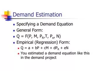
A. Steps in an analysis • (1) Specify variables: Quantity Demanded, Advertising, Income, Price, Other prices, Quality, Previous period demand, ... • (2) Obtain data: Cross sectional v. Time series • (3) Specify functional form of equation • Linear Yt = a + b X1t + g X2t + ut • Multiplicative Yt = a X1tb X2tg et • ln Yt = ln a + b ln X1t + g ln X2t + ut • (4) Estimate parameters • (5) Interpret results: economic and statistical
B. Regression Statistics from standard statistical packages (Minitab, SAS, Eviews, SPSS, etc.) • (1) Regression coefficients • (2) Standard error of regression coefficients, • t statistics, and p-values • (3) Coefficient of Determination (R2) • (4) F statistic • (5) Standard error of the estimate
C. Special Problems • Violating the assumptions of regression including • (1) Multicollinearity- highly correlated independent variables • (2) Heteroscedasticity- errors do not have the same variance • (3) Serial correlation- error in period t is correlated with error in period t + k • (4) Identification problems - data from interaction of supply and demand do not trace out demand relationship
Transit Example • Y P T I H • YEAR Riders Price Pop. Income Parking Rate • 1966 1200 15 1800 2900 50 • 1967 1190 15 1790 3100 50 • 1968 1195 15 1780 3200 60 • 1969 1110 25 1778 3250 60 • 1970 1105 25 1750 3275 60 • 1971 1115 25 1740 3290 70 • 1972 1130 25 1725 4100 75 • 1973 1095 30 1725 4300 75 • 1974 1090 30 1720 4400 75 • 1975 1087 30 1705 4600 80 • 1976 1080 30 1710 4815 80 • 1977 1020 40 1700 5285 80 • 1978 1010 40 1695 5665 85
Y P T I H • YEAR Riders Price Pop. Income Parking Rate • 1979 1010 40 1695 5800 100 • 1980 1005 40 1690 5900 105 • 1981 995 40 1630 5915 105 • 1982 930 75 1640 6325 105 • 1983 915 75 1635 6500 110 • 1984 920 75 1630 6612 125 • 1985 940 75 1620 6883 130 • 1986 950 75 1615 7005 150 • 1987 910 100 1605 7234 155 • 1988 930 100 1590 7500 165 • 1989 933 100 1595 7600 175 • 1990 940 100 1590 7800 175 • 1991 948 100 1600 8000 190 • 1992 955 100 1610 8100 200
Linear Transit Demand Riders = 85.4 – 1.62 price … Pr Elas = -1.62(100/955) in 1992
Multiplicative Transit Demand Ln Riders = exp(3.25)P-.14 …