Regression Analysis in Economics: An In-depth Guide
Learn about demand estimation, multiple regression analysis, and how to forecast demand using regression techniques. Understand coefficient of determination and evaluate regression coefficients. Dive into problems and solutions in regression analysis.


Regression Analysis in Economics: An In-depth Guide
E N D
Presentation Transcript
Demand Estimation • Regression Analysis • The Coefficient of Determination • Evaluating the Regression Coefficients • Multiple Regression Analysis • The Use of Regression Analysis to Forecast Demand • Additional Topics • Problems in the Use of Regression Analysis
Regression Analysis Regression Analysis: A statistical technique for finding the best relationship between a dependent variable and selected independent variables. • Simple regression – one independent variable • Multiple regression – several independent variables
Regression Analysis Dependent variable: • depends on the value of other variables • is of primary interest to researchers Independent variables: • used to explain the variation in the dependent variable
Regression Analysis Procedure • Specify the regression model • Obtain data on the variables • Estimate the quantitative relationships • Test the statistical significance of the results • Use the results in decision making
Regression Analysis Simple Regression Y = a + bX + u Y = dependent variable X = independent variable a = intercept b = slope u = random factor
Regression Analysis Data • Cross-sectional data provide information on a group of entities at a given time. • Time-series data provide information on one entity over time.
Regression Analysis The estimation of the regression equation involves a search for the best linear relationship between the dependent and the independent variable.
Regression Analysis Method of ordinary least squares (OLS): A statistical method designed to fit a line through a scatter of points is such a way that the sum of the squared deviations of the points from the line is minimized. Many software packages perform OLS estimation.
Regression Analysis Y = a + bX The intercept (a) and slope (b) of the regression line are referred to as the parameters or coefficients of the regression equation.
Coefficient of Determination Coefficient of determination (R2): A measure indicating the percentage of the variation in the dependent variable accounted for by variations in the independent variables. R2 is a measure of the goodness of fit of the regression model.
Coefficient of Determination Total sum of squares (TSS) • Sum of the squared deviations of the sample values of Y from the mean of Y. • TSS = sum(Yi-Y)2 • Yi = data (dependent variable) • Y = mean of the dependent variable • i = number of observations
Coefficient of Determination Regression sum of squares (RSS) • Sum of the squared deviations of the estimated values of Y from the mean of Y. • RSS = sum(Yi-Y)2 • Yi = estimated value of Y • Y = mean of the dependent variable • i = number of observations > >
Coefficient of Determination Error sum of squares (ESS) • Sum of the squared deviations of the sample values of Y from the estimated values of Y. • ESS = sum(Yi-Yi)2 • Yi = estimated value of Y • Yi = data (dependent variable) • i = number of observations > >
Coefficient of Determination • TSS : see segment AC • RSS: see segment BC • ESS: see segment AB
Coefficient of Determination R2 = RSS = 1 - ESS TSS TSS R2 measures the proportion of the total deviation of Y from its mean which is explained by the regression model.
Coefficient of Determination If R2 = 1 the total deviation in Y from its mean is explained by the equation.
Coefficient of Determination If R2 = 0 the regression equation does not account for any of the variation of Y from its mean.
Coefficient of Determination The closer R2 is to unity, the greater the explanatory power of the regression equation. An R2 close to 0 indicates a regression equation will have very little explanatory power.
Coefficient of Determination As additional independent variables are added, the regression equation will explain more of the variation in the dependent variable. This leads to higher R2 measures.
Coefficient of Determination Adjusted coefficient of determination k = number of independent variables n = sample size
Evaluating the Regression Coefficients In most cases, a sample from the population is used rather than the entire population. It becomes necessary to make inferences about the population based on the sample and to make a judgment about how good these inferences are.
Evaluating the Regression Coefficients An OLS regression line fitted through the sample points may differ from the true (but unknown) regression line.
Evaluating the Regression Coefficients How confident can a researcher be about the extent to which the regression equation for the sample truly represents the unknown regression equation for the population?
Evaluating the Regression Coefficients Each random sample from the population generates its own intercept and slope coefficients. To determine whether b (or a) is statistically different from 0 we conduct a t-test.
Two-tail test Null Hypothesis H0 : b = 0 Alternative Hypothesis Ha : b ≠ 0 One-tail test Null Hypothesis H0 : b > 0 (or b < 0) Alternative Hypothesis Ha : b < 0 (or b > 0) Evaluating the Regression Coefficients
Evaluating the Regression Coefficients Test statistic t = b – E(b) SEb b = estimated coefficient E(b) = b = 0 (Null hypothesis) SEb = standard error of the coefficient
Evaluating the Regression Coefficients Critical t-value depends on: • Degrees of freedom (d.f. = n – k – 1) • One or two-tailed test • Level of significance Use a t-table to determine the critical t-value.
Evaluating the Regression Coefficients Compare the t-value with the critical value. Reject the null hypothesis if the absolute value of the test statistic is greater than or equal to the critical t-value. Fail to reject the null hypothesis if the absolute value of the test statistic is less than the critical t-value.
Multiple Regression Analysis In multiple regression analysis the coefficients indicate the change in the dependent variable assuming the values of the other variables are unchanged.
Multiple Regression Analysis An additional test of statistical significance is called the F-test. The F-test measures the statistical significance of the entire regression equation rather than each individual coefficient.
Multiple Regression Analysis Null Hypothesis H0: b1 = b2 = b3 = … = bk = 0 No relationship exists between the dependent variable and the k independent variables for the population.
Multiple Regression Analysis • F-test statistic
Multiple Regression Analysis Critical F-value (F*) depends on: • Numerator degrees of freedom • (n.d.f. = k ) • Denominator degrees of freedom • (d.d.f = n-k-1) • Level of significance Use a F-table to determine the critical F-value.
Multiple Regression Analysis Compare the F-value with the critical value. • If F > F* • Reject Null Hypothesis • The entire regression model accounts for a statistically significant portion of the variation in the dependent variable.
Multiple Regression Analysis Compare the F-value with the critical value. • If F < F* • Fail to reject Null Hypothesis • There is no statistically significant relationship between the dependent variable and all of the independent variables.
The Use of Regression Analysis to Forecast Demand Forecast of dependent variable Y tn-k-1SEE SEE = Standard error of the estimate ±
Additional Topics Proxy variable: an alternative variable used in a regression when direct information in not available Dummy variable: a binary variable created to represent a non-quantitative factor.
Additional Topics The relationship between the dependent and independent variables may be nonlinear.
Additional Topics We could specify the regression model as quadratic regression model. Y = a +b1x + b2x2
Additional Topics We could also specify the regression model as power function. Y = axb or log Qd = log a + b(logX)
The estimation of demand may produce biased results due to simultaneous shifting of supply and demand curves. This is referred to as the identification problem. Advanced estimation techniques, such as two-stage least squares, are used to correct this problem. Problems
Problems If two independent variables are closely associated, it becomes difficult to separate the effects of each on the dependent variable. If the regression passes the F-test but fails the t-test for each coefficient, multicollinearity exists. A standard remedy is to drop one of the closely related independent variables from the regression.
Problems Autocorrelation occurs when the dependent variable deviates from the regression line in a systematic way. The Durbin-Watson statistic is used to identify the presence of autocorrelation. To correct autocorrelation consider: • Transforming the data into a different order of magnitude. • Introducing leading or lagging data