Download

1 / 30
430 likes | 2.08k Vues
Introduction to X-ray Pole Figures. L2 from 27-750, Advanced Characterization & Microstructural Analysis, A.D. (Tony) Rollett. Seminar 1, part A. How to Measure Texture. X-ray diffraction; pole figures; measures average texture at a surface (µms penetration); projection (2 angles) .

E N D
Introduction to X-ray Pole Figures L2 from 27-750, Advanced Characterization & Microstructural Analysis, A.D. (Tony) Rollett Seminar 1, part A
How to Measure Texture • X-ray diffraction; pole figures; measures average texture at a surface (µms penetration); projection (2 angles). • Neutron diffraction; type of data depends on neutron source; measures average texture in bulk (cms penetration in most materials) ; projection (2 angles). • Electron [back scatter] diffraction; easiest [to automate] in scanning electron microscopy (SEM); local surface texture (nms penetration in most materials); complete orientation (3 angles). • Optical microscopy: optical activity (plane of polarization); limited information (one angle).
Texture: Quantitative Description • Three (3) parameters needed to describe the orientation [of a crystal relative to the embedding body or its environment]. • Most common: 3 [rotation] Euler angles. • Most experimental methods [X-ray pole figures included] do not measure all 3 angles, so orientation distribution must be calculated. • Best representation: quaternions.
X-ray Pole Figures • X-ray pole figures are the most common source of texture information; cheapest, easiest to perform. • Pole figure:= variation in diffracted intensity with respect to direction in the specimen. • Representation:= map in projection of diffracted intensity. • Each PF is equivalent to a geographic map of a hemisphere (North pole in the center). • Map of crystal directions w.r.t. sample reference frame.
PF apparatus • From Wenk • Fig. 20: showing path difference between adjacent planes leading to destructive or constructive interference. • Fig. 21: pole figure goniometer for use with x-ray sources.
PF measurement • PF measured with 5-axis goniometer. • 2 axes used to set Bragg angle (choose a specific crystallographic plane with q/2q). • Third axis tilts specimen plane w.r.t. the focusing plane. • Fourth axis spins the specimen about its normal. • Fifth axis oscillates the Specimen under the beam. • N.B. deviations of relative intensities in a q/2q scan from powder file indicate texture.
Miller Indices • Cubic system: directions, [uvw], are equivalent to planes, (hkl). • Miller indices for a plane specify reciprocals of intercepts on each axis.
Miller Index Definition of Texture Component • The commonest method for specifying a texture component is the plane-direction. • Specify the crystallographic plane normal that is parallel to the specimen normal (e.g. the ND) and a crystallographic direction that is parallel to the long direction (e.g. the RD). (hkl) || ND, [uvw] || RD, or (hkl)[uvw]
Miller indices of a pole Miller indices are a convenient way to represent a direction or a plane normal in a crystal, based on integer multiples of the repeat distance parallel to each axis of the unit cell of the crystal lattice. This is simple to understand for cubic systems with equiaxed Cartesian coordinate systems but is more complicated for systems with lower crystal symmetry. Directions are simply defined by the set of multiples of lattice repeats in each direction. Plane normals are defined in terms of reciprocal intercepts on each axis of the unit cell. When a plane is written with parentheses, (hkl), this indicates a particular plane normal: by contrast when it is written with curly braces, {hkl}, this denotes a the family of planes related by the crystal symmetry. Similarly a direction written as [uvw] with square brackets indicates a particular direction whereas writing within angle brackets , <uvw> indicates the family of directions related by the crystal symmetry.
Pole Figure Example • If the goniometer is set for {100} reflections, then all directions in the sample that are parallel to <100> directions will exhibit diffraction.
Projection from Sphere to Plane • Projection of spherical information onto a flat surface • Equal area projection, or,Schmid projection • Equiangular projection, or,Wulff projection, more common in crystallography [Cullity] Obj/notation AxisTransformation Matrix EulerAngles Components
Stereographic Projections • Connect a line from the South pole to the point on the surface of the sphere. The intersection of the line with the equatorial plane defines the project point. The equatorial plane is the projection plane. The radius from the origin (center) of the sphere, r, where R is the radius of the sphere, and a is the angle from the North Pole vector to the point to be projected (co-latitude), is given by:r = R tan(a/2) • Given spherical coordinates (a), where the longitude is (as before), the Cartesian coordinates on the projection are therefore: (x,y) = r(cos, sin) = R tan(a/2)(cos, sin) • To obtain the spherical angles from [uvw], we calculate the co-latitude and longitude angles as: cosa = wtan = v/u Concept Params. Euler Normalize Vol.Frac. Cartesian Polar Components
Stereographic Projections StereographicEqual Area * Many texts, e.g. Cullity, show the plane touching the sphere at N: this changes the magnification factor for the projection, but not its geometry. [Kocks] Concept Params. Euler Normalize Vol.Frac. Cartesian Polar Components
The Stereographic Projection • Uses the inclination of the normal to the crystallographic plane: the points are the intersection of each crystal direction with a (unit radius) sphere. Obj/notation AxisTransformation Matrix EulerAngles Components
Standard Stereographic Projections • Pole figures are familiar diagrams. Standard Stereographic projections provide maps of low index directions and planes. • PFs of single crystals can be derived from SSTs by deleting all except one Miller index. • Construct {100}, {110} and {111} PFs for cube component.
Cube Component = {001}<100> {100} {111} {110} Think of the q-2q setting as acting as a filter on the standard stereographic projection,
Practical Aspects • Typical to measure three PFs for the 3 lowest values of Miller indices. • Why? • A single PF does not uniquely determine orientation(s), texture components because only the plane normal is measured, but not directions in the plane (2 out of 3 parameters). • Multiple PFs required for calculation of Orientation Distribution
Area Element, Volume Element • Spherical coordinates result in an area element, dA, whose magnitude depends on the declination (or co-latitude):dA = sinQdQdy Q dA d d [Kocks] Concept Params. Euler Normalize Vol.Frac. Cartesian Polar Components
Normalization • Normalization is the operation that ensures that “random” is equivalent to an intensity of one. • This is achieved by integrating the un-normalized intensity, f’(), over the full area of the pole figure, and dividing each value by the result, taking account of the solid area. Thus, the normalized intensity, f(), must satisfy the following equation, where the 2π accounts for the area of a hemisphere: Note that in popLA files, intensity levels are represented by i4 integers, so the random level = 100. Also, in .EPF data sets, the outer ring (typically, > 80°) is empty because it is unmeasurable; therefore the integration for normalization excludes this empty outer ring.
Summary • Microstructure contains far more than qualitative descriptions (images) of cross-sections of materials. • Most properties are anisotropic which means that it is critically important for quantitative characterization to include orientation information (texture). • Many properties can be modeled with simple relationships, although numerical implementations are (almost) always necessary.
Supplemental Slides • The following slides contain revision material about Miller indices from the first two lectures.
Corrections to Measured Data • Random texture [=uniform dispersion of orientations] means same intensity in all directions. • Background count must be subtracted. • X-ray beam becomes defocused at large tilt angles (> ~60°); measured intensity from random sample decreases towards edge of PF. • Defocusing correction required to increase the intensity towards the edge of the PF.
Defocussing • The combination of the q-2q setting and the tilt of the specimen face out of the focusing plane spreads out the beam on the specimen surface. • Above a certain spread, not all the diffracted beam enters the detector. • Therefore, at large tilt angles, the intensity decreases for purely geometrical reasons. • This loss of intensity must be compensated for, using the defocussing correction.
Defocusing Correction • Defocusing correction more important with decreasing 2q and narrower receiving slit.
popLA and the Defocussing Correction Values for correcting background Values for correcting data demo (from Cu1S40, smoothed a bit: UFK) 111 1000.00 999. 999. 999. 999. 999. 999. 999. 999. 999. 982.94 939.04 870.59 759.37 650.83 505.65 344.92 163.37 2.19 0 5 10 15 20 25 30 35 40 45 50 55 60 65 70 75 80 85 90 100.00 100.00 100.00 100.00 100.00 100.00 100.00 100.00 100.00 100.00 99.00 96.00 92.00 83.00 72.00 54.00 32.00 13.00 .00 TiltAngles 0 5 10 15 20 25 30 35 40 45 50 55 60 65 70 75 80 85 90 TiltAngles At each tilt angle, the data is multiplied by 1000/value
Miller <-> vectors • Miller indices [integer representation of direction cosines] can be converted to a unit vector, n: {similar for [uvw]}.
Direction Cosines • Definition of direction cosines: • The components of a unit vector are equal to the cosines of the angle between the vector and each (orthogonal, Cartesian) reference axis. • We can use axis transformations to describe vectors in different reference frames (room, specimen, crystal, slip system….)
Euler Angles, Animated e’3= e3=Zsample=ND [001] [010] zcrystal=e”’3= e”3 f1 ycrystal=e”’2 e”2 f2 e’2 e2=Ysample=TD xcrystal=e”’1 [100] F e’1 =e”1 e1=Xsample=RD
Equal Area Projection • Connect a line from the North Pole to the point to be projected. Rotate that line onto the plane tangent to the North Pole (which is the projection plane). The radius, r, of the projected point from the North Pole, where R is the radius of the sphere, and a is the angle from the North Pole vector to the point to be projected, is given by:r = 2R sin(a/2) • Given spherical coordinates (a), where the longitude is (as before), the Cartesian coordinates on the projection are therefore: (x,y) = r(cos, sin) = 2R sin(a/2)(cos, sin) Concept Params. Euler Normalize Vol.Frac. Cartesian Polar Components