Predation
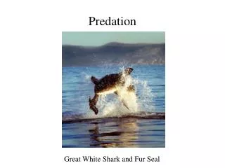
Predation. Predation – one species feeds on another enhances fitness of predator but reduces fitness of prey. ( +/– interaction). Charles Elton (1942).


Predation
E N D
Presentation Transcript
Predation – one species feeds on another enhances fitness of predator but reduces fitness of prey (+/– interaction)
Charles Elton (1942) British ecologist who studied mammalian population data. He concluded that oscillations were common and suggested that predators regulate prey populations. Cycles caused by predator –prey interactions predators prey
Lotka – Volterra Predation model Mathematicians who tried to model predator-prey interactions wondered: . - to what extent do predators cause these cyclic fluctuations (are they ½ responsible? Completely responsible?) - are other factors important? - do predators keep prey populations below K? (If so then no reason to believe completion is important because resources would not be limiting) - if predators are so efficient, why don’t the prey populations go extinct?
Predator-Prey Interaction Model Changes in prey population N = # of prey r1 = intrinsic rate of increase in prey populations k1 = constant that measures the ability of the prey to escape predators (0-1) P = # of predators r1N=density independent growth - k1 PN = reflects the negative effect of predators on prey
dN = - + r P k NP 2 2 dt Predator-Prey Interaction Model Changes in predator population r2 = death rate in predator population k2 = constant that measures the ability of the predators to capture prey (0-1) P = # of predators - r2P = negative of density independent growth (drag on predator populations Assumption: no density dependent effects (no carrying capacity, no competition) only predation
Predator-Prey Interaction Model This model did produce an oscillation between prey and predator populations (thus, it appeared to reflect natural situations). However, more complicated models showed that they were math. unstable. Gause : 1st test of model – observed two species of protozoans (prey and predator) grown on an oat medium. Predator always totally consumed the prey, then starved to death.
Predator-Prey Interaction Model Gause :By adding sediment to the oat medium (habitat complexity) for hiding places for the prey (paramecium). Predators starved to death, then the prey populations increased dramatically. Gause concluded that the cycles seen in nature are the result of constant migration, because he could not get coexistence in his experiments.
Carl B. Huffaker (1950’s) Insect ecologist Experimented with predators and their prey species that fed on commercially important citrus crops. He concluded that Gause’s experiments were too simple to reflect nature. Studied predator and prey mite spp. on oranges. Prey fed on oranges and predators fed on prey. Lab arenas had oranges in rectangular trays and densities of predators/prey were manipulated. Also increased habitat complexity by adding rubber balls and vasoline barriers. oranges only: predators ate prey and then starved to death. oranges, balls and vasoline:complexity allowed coexistence
C. S. Holling (1960’s) Conducted studies on the components of predatory interactions (acts among individual organisms) Worked with vertebrates and invertebrates (entomologist, concerned with the outbreaks of insects in forests which denuded trees.) Functional response – relationship between prey density and the rate at which an individual predator consumes prey Numerical response- increase in predator numbers with increases in prey abundance
Components of Functional Responses (for individual predators) • Rate of successful search • a. ratio of the speed of predator to prey • b. size of the field of reaction of the predator (distance at which the predator can perceive the prey) • c. success rate of capture (does a predator get a prey every time he encounters it)
Pumpkinseed Lepomis gibbosus Confer and Blades 1975 (L&O) Why are predators size-selective? Encounter frequency:Encounter of large prey is higher than small prey Reaction distance—how close to the fish does a prey item have to be for the fish to see it and react to (eat) it?
Reaction distance = radius of sphere Reaction distance translates to overall volume searched, which influences vulnerability of the prey Longer radius = higher encounter rate
Two types of Ceriodaphnia Big eye Small eye Artificially made small-eye morph more visible by feeding them india ink. Predation rate increased It is not just size that matters, it is overall visibility Zaret 1972 Fish always took the big-eye form.
Components of Functional responses (for individual predators) • Time available for hunting verses other activities • other activities necessary for an organism to carry on to reproduce is going to influence the amount of time available to hunt • a. avoiding other predators • b. time looking for a mate • c. patrolling a territory
Components of Functional Responses (for individual predators) 3. Time spent handling prey amount to time it takes to capture a prey after recognizing a potential food source a. pursuit of prey b. subduction of prey c. eating prey d. digesting prey 4. Hunger level– function of the size of the gut of the predator and the time spent in digestion and assimilation (rapid versus slow metabolsim)
Type I: Functional Response Linear increase; same assumptions as the Lotka-Votera growth models No examples of Type I functional response curve observed in natural systems
Type II: Functional Response Leveling off of # of prey eaten even though the # of prey increases (satiation of predators or time spent hunting prey) Holling found Type II curve with invertebrate predators
Type III: Functional Response Lag period: even as density of prey increases the # of prey eaten doesn’t increase dramatically (thought to result from the formation of search image by predators) These were all the results of laboratory experiments that Holling conducted. People later found a few examples of Type II and more examples of Type III.
Search image – when prey are rare there is no value in hunting for them. Only when the prey population increases above some threshold level does the predator form a search image and begin to recognize that prey item as a valuable food source. The predator then focuses on and exploits that food source heavily.
Numerical response – when there is a large increase in prey density, the predators present can become satiated as prey densities increase and the rate of prey eaten is not going to increase for each individual predators. However, if predators are added to the population increased exploitation of the prey can occur (due to immigration not reproduction)
Switching If predators exploit prey populations heavily and drive prey populations down, eventually prey densities will decline below some threshold value and predators will switch to another prey item. If switching occurs then more than one prey species can coexist(many studies have found switching to take place).
Murdoch (1960’s) Conducted the 1st switching experiments – examined gastropods that feed on mussels and barnacles and found that switching took place. -best candidate for switch occurred when the predator exhibited a weak preference for prey species
Prudent Predators Predators can drive prey pops. to extinction. But there is some optimal level of predation intensity that will maximize the # of predators without driving the prey extinct. It has been suggested that predators might “manage” prey populations and that this might explain why predators and prey usually coexist. Problem: individuals must cooperate with each other. But why not cheat? Evidence: predators can be prudent without “altruistic behavior” because exploitation of prey is determined by the ability of predators to capture them. And which individuals are usually removed from prey populations?
Back to the Rocky Intertidal • Early work by Connell (1970) • Conducted a 9 year study of barnacles and predatory whelks (San Juan Island, WA)
Juveniles barnacles Adult barnacles Predatory Whelks Observations
Results Midshore level: excluding whelks resulted in an adult population Lowshore: small whelks got into cages Model Model: Lower limit of adults caused by predation H1: Excluding predators in low areas leads to presence of adults Experiment: predator exclusion cages on a pier piling
Conclusion • Predation controls lower limit of barnacle population • Contrast with Connell (1961), where • competition controlled lower limit of Chthamalus • Reason for difference? • - predation reduced density below which competition could occur • - space not limiting
Lakes in North America • When fish introduced there were huge changes • - predators preferred the larger zooplankton • small zooplankton became dominant • large phytoplankton become abundant Brooks and Dodson 1965(over 1350 citations) Effects of predation on morphology, distribution and abundance • Change in size structure of prey population • (if predator prefers the largest individuals in a prey population) or there are shifts in the relative abundance of prey species (such that smaller species become quite abundant and the larger prey species becomes rare).
Effects of predation on morphology, distribution and abundance • 2. Decreases in overall diversity – if predators are very efficient at removing prey, they drive populations to extinction which reduces diversity • Increase in diversity– in simple systems with few prey species, one of which is a dominant competitor. If a predator prefers the dominant competitor it can reduce the number of the dominant competitor, allowing the inferior competitors to exist. • All three of these can occur in “ecological time” = one to a few generations
Paine 1966 • Effect of Pisaster on intertidal assemblage • 15 species coexist in intertidal • Food web: Pisaster starfish the dominant consumer
Experimental Design 8 x 2 m Plots in intertidal Control Pisaster removal Monitored changes over one year
Results Control plot: no change Removal plot: 80% barnacles (3 months) Mussels starting to dominate (1 yr) Species diversity decreased 15 to 8 spp. Predicted mussels would dominate available space
Conclusions • Pisaster interrupts successional process • After removal, superior competitor dominates Produced the concept of the “keystone predator” Limitations: no replication; did not examine smaller fauna (can be very diverse)
Keystone species paradigm Pisaster become known as a “keystone species” Paine (1966) cited 850 times 1970 –1979 Defined as “a single native species, high in the food web … which greatly modifies the species composition and physical appearance of the system” (Paine 1969)
Is the keystone a useful concept? Paine intended the term as metaphor – he rarely used it Others picked up on it -particularly conservation biologists (conserving keystones to maintain diversity) Problems: - identifying them - can be context dependent - may overlook other important species Criticized by Hurlburt (1997) and others
Menge (1994) Effects of Pisaster under different conditions Transplanted mussel clumps Hypothesis:Pisaster will consume mussels at all locations where it is present
Experimental Design Boiler Bay Strawberry Hill Sheltered Exposed Sheltered Exposed Pred No pred Pred No pred Pred No pred Pred No pred Turf Bare Replicates (n=5)
Take home message Predation can regulate assemblage structure - Directly: influences prey distribution - Indirectly: can mediate competition Keystone concept – beware of generality Results Pisaster more important at exposed sites Other sites: diffuse predation, with strong effect shared among species “Keystone” effect context dependent Why? – low productivity
Trophic Cascade in Kelp Forests When the keystone sea otter is removed, sea urchins overgraze kelp and destroy the kelp forest community. Figure 5.15b
Effects of predation on morphology, distribution and abundance • Morphological modifications – inference from observation • a. protective devices (spines on sea urchins; strong shells)
Effects of predation on morphology, distribution and abundance • Morphological modifications – inference from observation • b. mimicry – organisms that resemble unpalatable species (usually because they contain toxic compounds)
Effects of predation on morphology, distribution and abundance • Morphological modifications – inference from observation • c. crypsis – organisms match the color and shading of their habitats. Believed this morphology shaped by predatory pressure over time.
Artificial camouflage • Decorator crabs put algae on their backs, which increases their survival • In areas with Dictyota algae, crabs use this species for decoration, but rarely food
Optimal Foraging - types of feeding behaviors that would maximize food intake rate. Important because increased food intake results in larger and healthier organisms with more energy for growth and reproductive output. (maximize fitness) Is taking the largest prey item the best strategy?
Elner and Hughes (1978) Used predatory green crabs (Carcinus maenas) and mussels. Several different sizes of mussels were offered (small, medium and large). Feeding trials looked at the amount of energy/unit time.
Manipulation: Fixed the proportion of different sized mussels but varied the overall abundance (# of each size class in a given area) Observation: Proportion of each size class eaten under different abundances. Conclusion: The crabs are foraging in a size-selective manner AND they get more selective at higher abundances However, they still sample unprofitable size classes
Goss-Custard (1977) • Studied size selection of worms eaten by redshanks (Tringa totanus). Redshanks selected prey of 7mm more than any other size class even though prey of 8mm were more common. Thus, worms were eaten in proportion to their net energy benefit --not in relation to their abundance. • Also…. • When large #’s of worms available birds were selective • When small #’s of worms were available all were consumed • (take what you can get)
2. Optimal foraging—take the prey that provides the greatest energy return for cost of capture/handing. Werner and Hall (1974) Ecology With abundant prey, bigger is better Fed fish choice of three sizes of Daphniamagna