Chapter 7: The Normal Probability Distribution

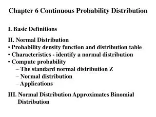
1. Chapter 7: The Normal Probability Distribution 7.1 Properties of the Normal Distribution 7.2 The Standard Normal Distribution 7.3 Applications of the Normal Distribution 7.4 Assessing Normality 7.5 The Normal Approximation to the Binomial Probability Distribution December 8, 2008 1

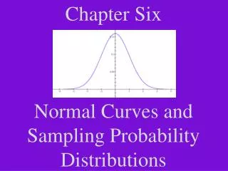
2. Properties of the Normal Distribution In this chapter we study a probability distribution for a continuous random variable, called the Normal Distribution. This distribution is studied for several reasons: It is a good model for the distribution of many different populations. (2) Several probability distributions (including some discrete probability distributions) can be approximated by a Normal Distribution. (3) It is bell-shaped and hence, the Empirical Rule applies. (4) Many inferential methods in statistics is based on the assumption that the population is distributed according to a Normal Distribution. Hence, it is ubiquitous. If you want to have detailed knowledge of only one probability distribution, then the Normal Distribution is one to study. Section 7.1

3. Continuous Random Variables • A continuous random variable has a continuum of possible values. • Examples: time, age, height and weight. • A continuous random variable has a continuous probability distribution that is a curve that is defined on the interval from which X takes its values.

4. Probability Distribution of a Continuous Random Variable Definition: Let X be a continuous random variable. Suppose that values of X, i.e., x, lie in an interval [a,b]. The probabilitydistributionofX is a function, f(x), that is define on [a,b], such that the area under the graph of f is equal to 1. The function, f(x), is also called the probabilitydensityfunction (PDF) of the distribution. Note: It is possible that either a and/or b are infinity.

5. Probabilities and Continuous Probability Distributions In the discrete case, we can extend the probability of x (say at x = 2) to the interval [1.5,2.5]. The probability for any x in [1.5,2.5] will be P(2). This probability is equal to the area of the rectangle whose base is the interval [1.5,2.5] and the height is P(2). This manner we can extend a discrete probability distribution to a continuous probability distribution that is defined on an intervals. For example, the probability for any x in [1.5,2.5] is P(2) which is area of the rectangle constructed above.

6. Area and Discrete Probability Distribution Recall: If x1 < x2 < …< xN, then P(x ≤ xk) = P(x1) + P(x2) + … + P(xk). From the histogram of the discrete probability distribution, the quantity, P(x1) + P(x2) + … + P(xk), is related to the area of the bars in the histogram. In fact, if the width of the bars are 1, then it is exactly the sum of the areas of the bars from x1 to xk. Hence, P(x ≤ xk) is an area “under the bar.” • Note: • P(x ≤ xN) = 1 • If m < n, then P(xm ≤ x ≤ xn) is the sum of the areas of the bars from xm to xn.

7. Probabilities and Continuous Probability Distributions For a continuous probability distribution, we generalize the ideas presented for the discrete probability distribution. Let us consider some interval [,] in the interval [a,b]. We want to associate a probability for x in the interval [,]. We define the probabilityforxintheinterval [,] as the area under the curve of f(x) and above the interval [,] .

8. Cumulative Probability Distribution

9. Continuous-Discrete Probability Distribution of a Random Variable Example:The random variable is the height of females in a certain population. As the number of possible outcomes for a random variable X becomes large, the discrete probability distribution can approach a continuous probability distribution. We can often approximate discrete probability distribution by continuous probability distributions.

10. Remark

11. Mean and Standard Deviation of a Continuous Probability Distribution

12. Summary of a Probability Distribution for a Continuous Random Variable

13. The Uniform Probability Distribution

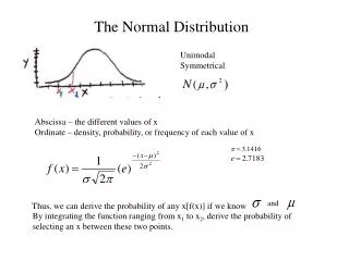
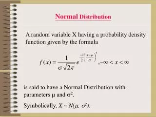
14. Normal Probability Distribution We now examine a particular probability distribution for a continuous random variable that takes all values of the real line. Remark: The function f(x) is called a probabilitydensityfunction and is abbreviated as PDF. We shall call the probability distribution, given by the above probability distribution function, the NormalDistribution.

15. Remark

16. Dependence on Mean and Standard Deviation  = 0 and  = 1  = 0 and  = 3  = 2 and  = 1  = -2 and  = 1 We will call the graph of f(x) the normaldensitycurve or simply, the normalcurve.

17. Computing the Probability Distribution Function for the Normal Curve • How can you calculate the function f(x) for different values of x? Once you have define  and , you use: • calculator • computer • tables

18. Facts about the Normal Distribution • Here are some properties of the graph of the normal density function f(x): • It is symmetric with respect to the line x =  • The highest value of the curve occurs when x = . • It has two points of inflection: x =  ± . A point of inflection is were a curve changes from being concave upward to concave downward or vice-versa. • The area under the curve is 1. • It highest value of f(x) (at x = ) changes with , but is always positive. • For some standard deviations, , the values of f(x) may be larger than 1.0 and hence, probability density function at a point, x, is not necessarily the probability, P(x).

19. Some Useful Facts about the Normal Distribution Function

20. Empirical Rule for the Normal Distribution • For the normal distribution and its curve, we have the following empirical rules for bell-shaped distributions: • Approximately 68% of the area under the curve lies in the interval [-, +]. • Approximately 95% of the area under the curve lies in the interval [-2, +2]. • Approximately 99.7% of the area under the curve lies in the interval [-3, +3]. • Recall: The empirical rule for bell-shaped distributions.

21. The Normal Cumulative Probability Distribution Definition: The CumulativeProbabilityDistribution, P(x ≤ ), is defined to be the area under the Normal Probability Density Function for x ≤ . The value of P(x ≤ ) is always between 0 and 1.

22. Fact about P(x ≤ ) Fact: The Normal Cumulative Probability Distribution (Normal CPD) of x gives the probability that x ≤ . For example, if X denotes the continuous random variable which is the weight of an individual randomly chosen from a population that obeys a normal distribution and x is the numerical value for this random variable, then P(x ≤ 180) is the probability that this individual weighs at least 180 pounds.

23. Cumulative Probability Distribution of an Interval Another Fact: The normal cumulative probability distribution for an interval [,] is the area under the curve and above the interval: P(≤ x ≤ ).

24. Example Suppose the replacement time of a particular brand of refrigerator is normally distributed with mean  = 14 years and standard deviation  = 2.5 years. Sketch a graph of the probability density function and the cumulative probability density function. (b) Shade the region in the graph of the probability density function that represents the probability that a randomly selected refrigerator will last at least 17 years. (c) What is the probability that it will last more than 17 years. (d) What is the probability that it will be replaced between 14 years and 16.5 years.

25. Calculation of the Cumulative Probability Distribution on the TI-83 • 2nd VARS (DISTR) key • Select normalcdf( [ENTER] • Complete entry e.g., normalcdf(-1.9,2.3,0.5,1.7) [ENTER] • Answer: 0.7761502183

26. z - score Recall: We introduce the concept of the z-score for an observation in a sample: z = (observation - mean)/(standard deviation) or letting observation = x, mean =  and standard deviation = , we have z = (x - )/. For example, when z = ±1, then x =  ± . When z = ±2, then x =  ± 2. In general, the z-score is a measure of how far is the observation (x) from the mean.

27. z-score and the Normal Distribution • Between z = -1 and z = 1, the values of x lie in the interval [-,+]. We know from the empirical rule, this is approximately 68% of the total area under the normal curve. • Between z = -2 and z = 2, the values of x lie in the interval [-2,+2]. We know from the empirical rule, this is approximately 95% of the total area under the normal curve. • Between z = -3 and z = 3, the values of x lie in the interval [-3,+3]. We know from the empirical rule, this is approximately 99.7% of the total area under the normal curve. • Hence, P(-≤ x ≤ +) is approximately 0.68, P(-2≤ x ≤ +2) is approximately 0.95, and P(-3≤ x ≤ +3) is approximately 0.997.

28. Standard Normal Distribution Definition: The normal distribution with  = 0 and  = 1 is called the StandardNormalDistribution.

29. The Standard Random Variable

30. Example

31. The Standard Normal Distribution We observed in the previous section that every Normal Distribution with mean  and standard deviation  can be converted to a Standard Normal Distribution by the change of random variable: z = (x - )/. Normal Distribution Standard Normal Distribution Section 7.2

32. Computing Probabilities with the Standard Normal Distribution

33. Example Example: The time between release from prison and conviction for another crime for individuals under the age of 40 is normally distributed (i.e., the probability of these events happen is governed by a Normal Distribution) with a mean of 30 months and a standard deviation of 6 months. Find the probability that an individual who has been released from prison will be convicted of another crime within 24 months. Solution: We want to calculate P(x ≤ 24) with  = 30 and  = 6. We can use the standard normal distribution by introducing the z-score. z = (x - 30)/6 or when x = 24, then z = (24 - 30)/6 = -1. Now P(z ≤ -1) = 0.1587. Hence, 15.87% of the prisoners will return within 2 years. Below are the probability density function (PDF) and the cumulative probability distribution (CPD). Notice that P(x < 0) is approximately zero.

34. Calculating P(a ≤ z ≤ b) from Tables

35. Inverse Problem: Given the value of P(z ≤ a), find a Suppose that we are given the value of P(z ≤ a) i.e., the area under a Standard Normal curve and we want to determine the value of a. Methods: Tables Calculator - invNorm

36. Inverse Problem: Given the value of P(-a ≤ z ≤ a), find a Suppose that we are given the value of P(-a ≤ z ≤ a) i.e., the area under a Standard Normal curve and we want to determine the value of a.

37. Inverse Problem: Given the value of P(z > a), find a Suppose that we are given the value of P(z > a) i.e., the area under a Standard Normal curve and we want to determine the value of a.

38. Applications of the Normal Distribution One important application of the Normal Distribution is the following. Suppose a variable x in a population (e.g., the height of individuals in Math 127A) is distributed according to a Normal Distribution with mean  and standard deviation . If we consider X to be a continuous random variable, then what is the probability that any randomly selected individual from the population will satisfy: a ≤ x ≤ b? That is, what is P(a ≤ x ≤ b)? Remark: We sometimes substitute the word “proportion” for probability. That is, what proportion of the population will the random variable x lie in the interval [a,b]? Section 7.3

39. Example The Accreditation Council for Graduate Medical Education found that average hours worked by medical residents was 81.7 hours per week with a standard deviation of 6.9 hours. Suppose that we assume that the number of hours per week worked by medical residents is distributed by a Normal Distribution with  = 81.7 and  = 6.9. (a) What is the probability that a medical resident will work more than 80 hours per week? (b) What is the probability that a randomly selected resident will work between 60 and 80 hours per week?

40. Example The Timken Company manufactures ball bearings with a mean diameter of 5 mm. Due to the manufacturing process there is some variation in the diameters of the ball bearings. It has been calculated that the distribution of diameters is normally distributed with a mean of 5 and a standard deviation of 0.02 mm. (a) What proportion of the ball bearings have diameters which are greater than 5.03 mm? (b) Any ball bearing that is smaller than 4.95 mm in diameter or greater than 5.05 mm is discarded. What proportion of ball bearings is discarded? (c) In one day, 30,000 ball bearings are manufactured. How many would you expect to be discarded in a day?

41. Assessing Normality Suppose that a variable of a population X is distributed according to an unknown distribution. Is there a way that we can test if this unknown distribution is actually a Normal Distribution? One Approach: Take a large finite sample from the population and create a histogram to see if the histogram has the characteristics of a Normal Distribution i.e., it is bell-shaped. However, being bell-shaped does not mean that it is a Normal Distribution. Section 7.4

42. Another Approach TI-83: NormProbPlot

43. Example Data:{0.533226, 2.73637, 2.76095, 2.83428, 2.62008, 1.82784, 1.31128, 1.87577, 0.70117, 3.09077, 2.47481, 2.09632, 2.22858, 2.23172, 1.76795, 0.153967, 1.19405, 2.70018, 1.66897, 0.583992} Sorted Data: {0.153967, 0.533226, 0.583992, 0.70117, 1.19405, 1.31128, 1.66897, 1.76795, 1.82784, 1.87577, 2.09632, 2.22858, 2.23172, 2.47481, 2.62008, 2.70018, 2.73637, 2.76095, 2.83428, 3.09077} Normal Scores: {-1.86824, -1.40341, -1.12814, -0.919136, -0.744143, -0.589456, -0.447768, -0.314572, -0.186756, -0.0619316, 0.0619316, 0.186756, 0.314572, 0.447768, 0.589456, 0.744143, 0.919136, 1.12814, 1.40341, 1.86824} n = 20 Note: Data was generated by a Normal Distribution with  = 2 and  = 0.75.

44. Example Data:{-8.21923, -2.74515, -0.386428, -0.677152, 4.02123, -0.826667, 9.17761, 6.45027, -2.31864, 6.53159, 7.68041, -1.54977, -0.988243, 3.35719, 5.98133, 4.44442, 4.03768, 9.3086, 6.4066, -9.51397, -6.42983, 1.88659, -1.5584, 6.85724, -8.2106, -5.36826, 8.82803, -2.46561, -2.23184, 5.45841} Sorted Data: {-9.51397, -8.21923, -8.2106, -6.42983, -5.36826, -2.74515, -2.46561, -2.31864, -2.23184, -1.5584, -1.54977, -0.988243, -0.826667, -0.677152, -0.386428, 1.88659, 3.35719, 4.02123, 4.03768, 4.44442, 5.45841, 5.98133, 6.4066, 6.45027, 6.53159, 6.85724, 7.68041, 8.82803, 9.17761, 9.3086} Normal Scores: {-2.04028, -1.60982, -1.36087, -1.17581, -1.02411, -0.892918, -0.775547, -0.668002, -0.567686, -0.472789, -0.381976, -0.294213, -0.208664, -0.124617, -0.0414437, 0.0414437, 0.124617, 0.208664, 0.294213, 0.381976, 0.472789, 0.567686, 0.668002, 0.775547, 0.892918, 1.02411, 1.17581, 1.36087, 1.60982, 2.04028} n = 30 Note: Data was generated by a Uniform Distribution on the interval [-9,9].

45. Example Data:{0.00881683, 0.295109, 2.71993, 0.0275762, 1.15885, 1.01363, 0.295519, 0.639201, 0.602931, 0.446441, 0.0801617, 0.580694, 0.367919, 0.477032, 0.197738, 0.16514, 1.43215, 0.305959, 0.269021, 0.359607} Sorted Data: {0.00881683, 0.0275762, 0.0801617, 0.16514, 0.197738, 0.269021, 0.295109, 0.295519, 0.305959, 0.359607, 0.367919, 0.446441, 0.477032, 0.580694, 0.602931, 0.639201, 1.01363, 1.15885, 1.43215, 2.71993} Normal Scores: {-1.86824, -1.40341, -1.12814, -0.919136, -0.744143, -0.589456, -0.447768, -0.314572, -0.186756, -0.0619316, 0.0619316, 0.186756, 0.314572, 0.447768, 0.589456, 0.744143, 0.919136, 1.12814, 1.40341, 1.86824} n = 20 Note: Data was generated by a non-Normal Distribution.

46. The Normal Approximation to the Binomial Probability Distribution Section 7.5

47. Example According to the Commerce Department in 2004, 20% of U.S. households had some type of high-speed internet connection (cable, DSL, satellite). Suppose 80 U.S. households are selected at random. What is the probability that exactly 15 households of the 80 will have a high-speed internet connection?