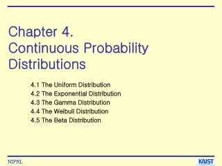
Chapter 6 Introduction to Continuous Probability Distributions
Business Statistics. Chapter 6 Introduction to Continuous Probability Distributions. Chapter Goals. After completing this chapter, you should be able to: Find probabilities using a normal distribution table and apply the normal distribution to business problems

Chapter 6 Introduction to Continuous Probability Distributions
E N D
Presentation Transcript
Business Statistics Chapter 6Introduction to Continuous Probability Distributions Tran Van Hoang - hoangtv@ftu.edu.vn - Business Statistics
Chapter Goals After completing this chapter, you should be able to: • Find probabilities using a normal distribution table and apply the normal distribution to business problems • Recognize when to apply the uniform and exponential distributions Tran Van Hoang - hoangtv@ftu.edu.vn - Business Statistics
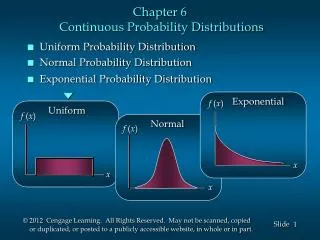
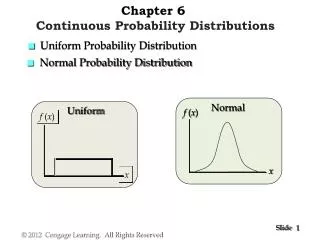
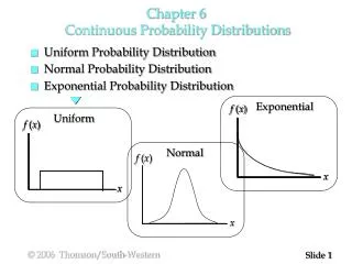
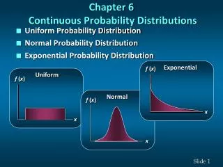
Probability Distributions Probability Distributions Discrete Probability Distributions Continuous Probability Distributions Binomial Normal Poisson Uniform Hypergeometric Exponential Tran Van Hoang - hoangtv@ftu.edu.vn - Business Statistics
Continuous Probability Distributions • A continuous random variable is a variable that can assume any value on a continuum (can assume an uncountable number of values) • thickness of an item • time required to complete a task • temperature of a solution • height, in inches • These can potentially take on any value, depending only on the ability to measure accurately. Tran Van Hoang - hoangtv@ftu.edu.vn - Business Statistics
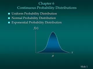
The Normal Distribution Probability Distributions Continuous Probability Distributions Normal Uniform Exponential Tran Van Hoang - hoangtv@ftu.edu.vn - Business Statistics
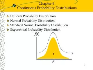
The Normal Distribution • ‘Bell Shaped’ • Symmetrical • Mean, Median and Mode are Equal Location is determined by the mean, μ Spread is determined by the standard deviation, σ The random variable has an infinite theoretical range: + to f(x) σ x μ Mean = Median = Mode Tran Van Hoang - hoangtv@ftu.edu.vn - Business Statistics
Many Normal Distributions By varying the parametersμand σ, we obtain different normal distributions Tran Van Hoang - hoangtv@ftu.edu.vn - Business Statistics
The Normal Distribution Shape f(x) Changingμ shifts the distribution left or right. Changingσincreases or decreases the spread. σ μ x Tran Van Hoang - hoangtv@ftu.edu.vn - Business Statistics
Finding Normal Probabilities Probability is the area under thecurve! Probability is measured by the area under the curve f(x) ) P ( a x b x a b Tran Van Hoang - hoangtv@ftu.edu.vn - Business Statistics
Probability as Area Under the Curve The total area under the curve is 1.0, and the curve is symmetric, so half is above the mean, half is below f(x) 0.5 0.5 μ x Tran Van Hoang - hoangtv@ftu.edu.vn - Business Statistics
Empirical Rules μ ± 1σencloses about 68% of x’s What can we say about the distribution of values around the mean? There are some general rules: f(x) σ σ x μ-1σ μ μ+1σ 68.26% Tran Van Hoang - hoangtv@ftu.edu.vn - Business Statistics
The Empirical Rule (continued) • μ ± 2σcovers about 95% of x’s • μ ± 3σcovers about 99.7% of x’s 3σ 3σ 2σ 2σ μ x μ x 95.44% 99.72% Tran Van Hoang - hoangtv@ftu.edu.vn - Business Statistics
Importance of the Rule • If a value is about 2 or more standard deviations away from the mean in a normal distribution, then it is far from the mean • The chance that a value that far or farther away from the mean is highly unlikely, given that particular mean and standard deviation Tran Van Hoang - hoangtv@ftu.edu.vn - Business Statistics
The Standard Normal Distribution Also known as the “z” distribution Mean is defined to be 0 Standard Deviation is 1 f(z) 1 z 0 Values above the mean have positive z-values, values below the mean have negative z-values Tran Van Hoang - hoangtv@ftu.edu.vn - Business Statistics
The Standard Normal Any normal distribution (with any mean and standard deviation combination) can be transformed into the standard normaldistribution (z) Need to transform x units into z units Tran Van Hoang - hoangtv@ftu.edu.vn - Business Statistics
Translation to the Standard Normal Distribution Translate from x to the standard normal (the “z” distribution) by subtracting the mean of x and dividing by its standard deviation: Tran Van Hoang - hoangtv@ftu.edu.vn - Business Statistics
Example If x is distributed normally with mean of 100 and standard deviation of 50, the z value for x = 250is This says that x = 250 is three standard deviations (3 increments of 50 units) above the mean of 100. Tran Van Hoang - hoangtv@ftu.edu.vn - Business Statistics
Comparing x and z units μ= 100 σ= 50 100 250 x 0 3.0 z Note that the distribution is the same, only the scale has changed. We can express the problem in original units (x) or in standardized units (z) Tran Van Hoang - hoangtv@ftu.edu.vn - Business Statistics
The Standard Normal Table The Standard Normal table in the textbook (Appendix D) gives the probability from the mean (zero) up to a desired value for z .4772 Example: P(0 < z < 2.00) = .4772 z 0 2.00 Tran Van Hoang - hoangtv@ftu.edu.vn - Business Statistics
The Standard Normal Table The value within the table gives the probability from z = 0 up to the desired z value (continued) The columngives the value of z to the second decimal point The row shows the value of z to the first decimal point . . . 2.0 .4772 P(0 < z < 2.00) = .4772 2.0 Tran Van Hoang - hoangtv@ftu.edu.vn - Business Statistics
General Procedure for Finding Probabilities • Draw the normal curve for the problem in terms of x • Translate x-values to z-values • Use the Standard Normal Table To find P(a < x < b) when x is distributed normally: Tran Van Hoang - hoangtv@ftu.edu.vn - Business Statistics
Z Table example Suppose x is normal with mean 8.0 and standard deviation 5.0. Find P(8 < x < 8.6) Calculate z-values: 8 8.6 x 0 0.12 Z P(8 < x < 8.6) = P(0 < z < 0.12) Tran Van Hoang - hoangtv@ftu.edu.vn - Business Statistics
Z Table example Suppose x is normal with mean 8.0 and standard deviation 5.0. Find P(8 < x < 8.6) (continued) • = 8 = 5 • = 0 = 1 x z 8 8.6 0 0.12 P(8 < x < 8.6) P(0 < z < 0.12) Tran Van Hoang - hoangtv@ftu.edu.vn - Business Statistics
Solution: Finding P(0 < z < 0.12) Standard Normal Probability Table (Portion) P(8 < x < 8.6) = P(0 < z < 0.12) .02 z .00 .01 .0478 .0000 0.0 .0040 .0080 .0398 .0438 .0478 0.1 0.2 .0793 .0832 .0871 Z 0.00 0.3 .1179 .1217 .1255 0.12 Tran Van Hoang - hoangtv@ftu.edu.vn - Business Statistics
Finding Normal Probabilities • Suppose x is normal with mean 8.0 and standard deviation 5.0. • Now Find P(x < 8.6) Z 8.0 8.6 Tran Van Hoang - hoangtv@ftu.edu.vn - Business Statistics
Finding Normal Probabilities (continued) • Suppose x is normal with mean 8.0 and standard deviation 5.0. • Now Find P(x < 8.6) .0478 .5000 P(x < 8.6) = P(z < 0.12) = P(z < 0) + P(0 < z < 0.12) = .5 + .0478 = .5478 Z 0.00 0.12 Tran Van Hoang - hoangtv@ftu.edu.vn - Business Statistics
Upper Tail Probabilities • Suppose x is normal with mean 8.0 and standard deviation 5.0. • Now Find P(x > 8.6) Z 8.0 8.6 Tran Van Hoang - hoangtv@ftu.edu.vn - Business Statistics
Upper Tail Probabilities (continued) • Now Find P(x > 8.6)… P(x > 8.6) = P(z > 0.12) = P(z > 0) - P(0 < z < 0.12) = .5 - .0478 = .4522 .0478 .5000 .50 - .0478 = .4522 Z Z 0 0 0.12 0.12 Tran Van Hoang - hoangtv@ftu.edu.vn - Business Statistics
Lower Tail Probabilities • Suppose x is normal with mean 8.0 and standard deviation 5.0. • Now Find P(7.4 < x < 8) Z 8.0 7.4 Tran Van Hoang - hoangtv@ftu.edu.vn - Business Statistics
Lower Tail Probabilities (continued) Now Find P(7.4 < x < 8)… The Normal distribution is symmetric, so we use the same table even if z-values are negative: P(7.4 < x < 8) = P(-0.12 < z < 0) = .0478 .0478 Z 8.0 7.4 Tran Van Hoang - hoangtv@ftu.edu.vn - Business Statistics
Normal Probabilities in PHStat We can use Excel and PHStat to quickly generate probabilities for any normal distribution We will find P(8 < x < 8.6) when x is normally distributed with mean 8 and standard deviation 5 Tran Van Hoang - hoangtv@ftu.edu.vn - Business Statistics
PHStat Dialogue Box Select desired options and enter values Tran Van Hoang - hoangtv@ftu.edu.vn - Business Statistics
PHStat Output Tran Van Hoang - hoangtv@ftu.edu.vn - Business Statistics
Exercises • 6-1. For a normally distributed population with μ=200 and σ=20, determine the standardized z-value for each of the following: • X=225 • X=190 • X=240 • 6-2. For a standardized normal distribution, calculate the following probabilities: • P(z <1.5) • P(z>0.85) • P(-1.28<z<1.75) Tran Van Hoang - hoangtv@ftu.edu.vn - Business Statistics
Exercises • 6-3. For a standardized normal distribution, calculate the following probabilities: • P(0.00 < z ≤ 2.33) • P(-1.00 < z ≤ 1.00) • P(1.78 < z < 2.34) • 6-4. For a standardized normal distribution, determine a value, say z0, so that • P(0 < z < z0) = 0.4772 • P(-z0 ≤ z < 0) = 0.45 • P(-z0≤ z z0) ≤ 0.95 • P(z > z0) = 0.025 • P(z < z0) = 0.01 Tran Van Hoang - hoangtv@ftu.edu.vn - Business Statistics
Exercises 6-7. For the following normal distributions with parameters as specified, calculate the required probabilities: a. μ=5,σ=2; calculate P(0 < x < 8). b. μ=5,σ=4; calculate P(0 < x < 8). c. μ=3,σ=2; calculate P(0 < x < 8). d. μ=4,σ=3; calculate P(x > 1). e. μ=0,σ=3; calculate P(x > 1). Tran Van Hoang - hoangtv@ftu.edu.vn - Business Statistics
The Uniform Distribution Probability Distributions Continuous Probability Distributions Normal Uniform Exponential Tran Van Hoang - hoangtv@ftu.edu.vn - Business Statistics
The Uniform Distribution • The uniform distribution is a probability distribution that has equal probabilities for all possible outcomes of the random variable Tran Van Hoang - hoangtv@ftu.edu.vn - Business Statistics
The Uniform Distribution (continued) The Continuous Uniform Distribution: f(x) = where f(x) = value of the density function at any x value a = lower limit of the interval b = upper limit of the interval Tran Van Hoang - hoangtv@ftu.edu.vn - Business Statistics
Uniform Distribution Example: Uniform Probability Distribution Over the range 2 ≤ x ≤ 6: 1 f(x) = = .25 for 2 ≤ x ≤ 6 6 - 2 f(x) .25 x 2 6 Tran Van Hoang - hoangtv@ftu.edu.vn - Business Statistics
The Exponential Distribution Probability Distributions Continuous Probability Distributions Normal Uniform Exponential Tran Van Hoang - hoangtv@ftu.edu.vn - Business Statistics
The Exponential Distribution • Used to measure the time that elapses between two occurrences of an event (the time between arrivals) • Examples: • Time between trucks arriving at an unloading dock • Time between transactions at an ATM Machine • Time between phone calls to the main operator Tran Van Hoang - hoangtv@ftu.edu.vn - Business Statistics
The Exponential Distribution • The probability that an arrival time is equal to or less than some specified time a is where 1/ is the mean time between events Note that if the number of occurrences per time period is Poisson with mean , then the time between occurrences is exponential with mean time 1/ Tran Van Hoang - hoangtv@ftu.edu.vn - Business Statistics
Exponential Distribution (continued) • Shape of the exponential distribution f(x) = 3.0 (mean = .333) = 1.0 (mean = 1.0) • = 0.5 (mean = 2.0) x Tran Van Hoang - hoangtv@ftu.edu.vn - Business Statistics
Example Example: Customers arrive at the claims counter at the rate of 15 per hour (Poisson distributed). What is the probability that the arrival time between consecutive customers is less than five minutes? • Time between arrivals isexponentially distributed with mean time between arrivals of 4 minutes (15 per 60 minutes, on average) • 1/ = 4.0, so = .25 • P(x < 5) = 1 - e-a = 1 – e-(.25)(5) = .7135 Tran Van Hoang - hoangtv@ftu.edu.vn - Business Statistics
Chapter Summary • Reviewed key discrete distributions • binomial, poisson, hypergeometric • Reviewed key continuous distributions • normal, uniform, exponential • Found probabilities using formulas and tables • Recognized when to apply different distributions • Applied distributions to decision problems Tran Van Hoang - hoangtv@ftu.edu.vn - Business Statistics