Understanding Continuous and Discrete Probability Distributions
This chapter explores the key concepts of continuous and discrete probability distributions. It illustrates how probabilities are represented using bar graphs for discrete values and under curves for continuous distributions. Figures detail Maria's commute time distribution, and the properties of normal distributions, including the empirical rule covering one, two, and three standard deviations. The chapter also addresses z-scores, the standard normal distribution, and the exponential distribution, providing insights into calculations for probabilities and expected values.

Understanding Continuous and Discrete Probability Distributions
E N D
Presentation Transcript
Figure 6.1 A Discrete Probability Distribution Probability is represented by the height of the bar. P(x) 1 2 3 4 5 6 7 x Holes or breaks between values
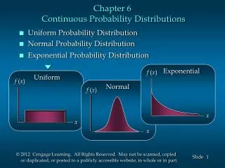
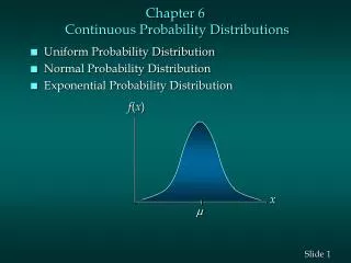
f(x) Probability is represented by area under the curve. x No holes or breaks along the x axis Figure 6.2 A Continuous Probability Distribution
f(x) 1/20 62 72 82 x (commute time in minutes) Figure 6.3 Maria’s Commute Time Distribution
f(x) 1/20 62 64 67 82 x (commute time in minutes) Figure 6.4 Computing P(64 <x< 67) Probability = Area = Width x Height= 3 x 1/20 = .15 or 15%
Total Area = 20 x 1/20 = 1.0 1/20 62 82 20 Figure 6.5 Total Area = 1.0 1/20
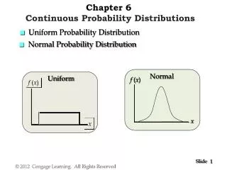
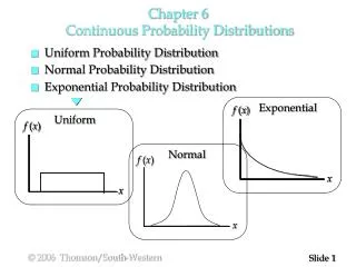
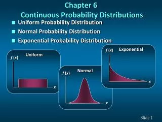
Uniform Probability Density Function (6.1) 1/(b-a) for a<x<b f(x) = 0 everywhere else
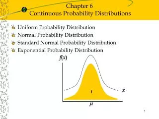
m Figure 6.7 The Bell-Shaped Normal Distribution Mean is m Standard Deviation is s x
Normal Distribution Properties • Approximately 68.3% of the values in a normal distribution will be within one standard deviation of the distribution mean, m. • Approximately 95.5% of the values in a normal distribution will be within two standard deviations of the distribution mean, m. • Approximately 99.7% of the values (nearly all of them) in a normal distribution will be found within three standard deviations of the distribution mean, m.
.683 m-1s m m+1s Figure 6.8 Normal Area for m+ 1s
.955 Figure 6.9 Normal Area for m+ 2s m-2s m m+2s
.997 m-3s m m+3s Figure 6.10 Normal Area for m+ 3s
Figure 6.11 Area in a Standard Normal Distribution for a z of +1.2 .3849 0 1.2 z
m =50 s = 4 .3944 50 55 x (diameter) 0 1.25 z Figure 6.12 P(50 <x< 55)
Figure 6.13 P(x> 58) m =50 s = 4 .0228 .4772 50 58 x(diameter) 0 2.0 z
.2734 .4332 m = 50 s = 4 47 50 56 x(diameter) -.75 0 1.5 z Figure 6.14 P(47 < x < 56)
m = 50 s = 4 .3413 .4772 50 54 58 x (diameter) 0 1.0 2.0 z Figure 6.15 P(54 < x < 58)
Figure 6.16 Finding the z score for an Area of .25 .2500 0 ? z
Exponential Probability (6.7) Density Function f(x) =
Figure 6.17 Exponential Probability Density Function f(x) f(x) =l/elx x
Calculating Area for the (6.8) Exponential Distribution P(x >a) =
f(x) P(x>a) = 1/ela x a Figure 6.18 Calculating Areas for the Exponential Distribution
f(x) P(1.0 <x< 1.5) x 1.0 1.5 Figure 6.19 Finding P(1.0 <x< 1.5)
f(x) P(x> 1.0) = .1354 P(x> 1.5) = .0498 x 1.0 1.5 Figure 6.20 Finding P(1.0 <x< 1.5)
Expected Value for the (6.9) Exponential Distribution E(x) =
Standard Deviation for the (6.11)Exponential Distribution s = =