Efficient 2D Heat Simulation of SPE-10 Reservoir Using Linear System Solvers in MATLAB
This MATLAB code simulates a 2D heat transfer model based on the SPE-10 benchmark case. It resolves linear systems using direct and iterative methods such as Gaussian elimination, LU decomposition, and preconditioned conjugate gradient (PCG). The model focuses on a reservoir with heterogeneous permeability distributed over a Cartesian grid, employing an injection and production well located at opposite corners. The program handles boundary conditions effectively while solving for node values and time evolution, making it suitable for large-scale simulation of reservoir behavior.

Efficient 2D Heat Simulation of SPE-10 Reservoir Using Linear System Solvers in MATLAB
E N D
Presentation Transcript
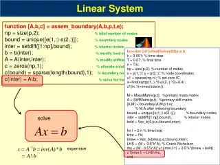
Linear System function [A,b,c] = assem_boundary(A,b,p,t,e); np = size(p,2); % total number of nodes bound = unique([e(1,:) e(2,:)]); % boundary nodes inter = setdiff([1:np],bound); % interior nodes b = b(inter); % modify load vector A = A(inter,inter); % modify stiffness matrix c = zeros(np,1); % allocate solution vector c(bound) = sparse(length(bound),1); % boundary nodes solution c(inter) = A\b; % solve for free node values function [u1]=HeatSolver2D(p,e,t) k = 0.001; % time step T = 0.07; % final time n = T/k; np = size(p,2); % number of nodes x = p(1,:)'; y = p(2,:)'; % node coordinates u1 = sparse(np,n); % set zero IC ix=find(sqrt(p(1,:).^2+p(2,:).^2)<0.4); u1(ix,1)=ones(size(ix)); M = MassMatrix(p,t); %primary mass matrix A = StiffMatrix(p,t); %primary stiff matrix [A,M] = boundary(A,M,p,t,e); % M,A after imbosing boundary bound = unique([e(1,:) e(2,:)]); % boundary nodes inter = setdiff([1:np],bound); % interior nodes bold = Vec_b(0,p,e,t,bound,inter); for l = 2:n % time loop time = l*k; bnew = Vec_b(time,p,e,t,bound,inter); LHS = (M + 0.5*k*A); % Crank-Nicholson rhs = (M - 0.5*k*A)*u1(inter,l-1) + 0.5*k*(bnew + bold); u1(inter,l) = LHS\rhs; end solve expensive
MATLAB code for SPE-10 I P 10% 90% SPE-10 with an injection and a production well in the lower-left and upper-right corners, respectively. This code simulate two horizontal slices of Model 2 from the 10th SPE Comparative Solution Project. which is publicly available on the net. The model dimensions are 1200 × 2200 × 170 (ft) and the reservoir is described by a heterogeneous distribution over a regular Cartesian grid with 60×220×85 grid-blocks. We pick the top layer, in which the permeability is smooth, and the bottom layer. For both layers, the permeabilities range over at least six orders of magnitude. To drive a flow in the two layers, we impose an injection and a production well in the lower-left and upper-right corners, respectively. MFEM MATLAB code applied to the top layer of the SPE-10 test case
MATLAB commands tic; factorial(21); toc
Linear System We want to solve the following linear system 2 classes of methods Direct Methods Iterative Methods Gaussian Elimination LU, Choleski These methods generate a sequence of approximate solutions
observations made by Horst Simon [173]. He predicted that by now we will have to solve routinely linear problems with some 5 × 10^9 unknowns. From extrapolation of the CPU times observed for a characteristic model problem, he estimated the CPU time for the most efficient direct method as 520 040 years, provided that the computation can be carried out at a speed of 1 TFLOPS. On the other hand, the extrapolated guess for the CPU time with preconditioned conjugate gradients, still assuming a processing speed of 1 TFLOPS, is 575 seconds. ‘flops’ floating point operations. Each addition, subtraction, multiplication, division, or square root counts as one flop.
Linear System We want to solve the following linear system 2 classes of methods Direct Methods Iterative Methods Krylov subspace others splitting Jacobi, GS, SOR,.. PCG, MINRES, GMRES, …
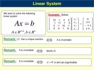
Linear System We want to solve the following linear system Example: Solve: 10 -1 2 0 -1 11 -1 3 2 -1 10 -1 0 3 -1 8 Remark: (1) has a unique solution A is invertable Remark: A is invertable det(A)=0 Remark: A is invertable
Linear System We want to solve the following linear system Remark: Definition: Example:
Iterative Method These methods generate a sequence of approximate solutions Remark:
Splittings and Convergence DEF: with eigenvalues spectral radius of A is defined to be DEF: Splitting A large family of iteration
Splittings and Convergence A large family of iteration Diagonal Lower Upper Jacobi: Gauss-Seidel:
Jacobi Method Consider 4x4 case Example 10 -1 2 0 -1 11 -1 3 2 -1 10 -1 0 3 -1 8
Jacobi Method 0.6000 1.0473 0.9326 1.0152 0.9890 2.2727 1.7159 2.0533 1.9537 2.0114 -1.1000 -0.8052 -1.0493 -0.9681 -1.0103 1.8750 0.8852 1.1309 0.9738 1.0214 11.3537 4.9910 2.0299 0.8911 0.3686 1.0032 0.9981 1.0006 0.9997 1.0001 1.9922 2.0023 1.9987 2.0004 1.9998 -0.9945 -1.0020 -0.9990 -1.0004 -0.9998 0.9944 1.0036 0.9989 1.0006 0.9998 0.1605 0.0671 0.0290 0.0122 0.0053
Gauss Seidel Method Note that in the Jacobi iteration one does not use the most recently available information. 0.6000 1.0302 1.0066 1.0009 1.0001 2.3273 2.0369 2.0036 2.0003 2.0000 -0.9873 -1.0145 -1.0025 -1.0003 -1.0000 0.8789 0.9843 0.9984 0.9998 1.0000 5.6930 0.4300 0.0662 0.0082 0.0009
Gauss Seidel Method Jacobi iteration for general n: Gauss-Seidel iteration for general n:
Splittings and Convergence A large family of iteration THM:
Splittings and Convergence Example: 10 -1 2 0 -1 11 -1 3 2 -1 10 -1 0 3 -1 8 10 11 10 8 -1 2 -1 0 3 -1 -1 2 0 -1 3 -1 10 -1 2 0 -1 11 -1 3 2 -1 10 -1 0 3 -1 8 Jacobi: U=triu(A,1) L=tril(A,-1) D=diag(diag(A)) eig(inv(M)*N) -0.4264 -0.1040 0.1860 0.3445 GS: 0 0 0.0839 - 0.0322i 0.0839 + 0.0322i
Splittings and Convergence A large family of iteration Remarks: THM: Proof: (Golub p511)
Splittings and Convergence THM: Proof: (Golub p512) show that all eigenvalues are less than one. Positive Definite Symmetric Stiffness Matrix Mass Matrix
Splittings and Convergence DEF: IF Example: THM:
Successive over Relaxation The Gauss-Seidel iteration is very attractive because of its simplicity. Unfortunately, if the spectral radius is close to one, then convergence is vey slow. One solution for this Successive over Relaxation GS:
Successive over Relaxation Example: Successive over Relaxation 10 -1 2 0 -1 11 -1 3 2 -1 10 -1 0 3 -1 8
Successive over Relaxation Successive over Relaxation Example: 10 -1 2 0 -1 11 -1 3 2 -1 10 -1 0 3 -1 8 0.6180 1.0553 1.0055 2.3988 2.0273 2.0004 -1.0132 -1.0211 -1.0014 0.8743 0.9905 1.0000
MATLAB CODE Ex: Write a Matlab function for Jacobi Jacobi iteration for general n: function [sol,X]=jacobi(A,b,x0) n=length(b); maxiter=10; x=x0; for k=1:maxiter for i=1:n sum1=0; for j=1:i-1 sum1=sum1+A(i,j)*x(j); end sum2=0; for j=i+1:n sum2=sum2+A(i,j)*x(j); end xnew(i)=(b(i)-sum1-sum2)/A(i,i) end X(1:n,k)=xnew; x=xnew; end sol=xnew;
MATLAB CODE Ex: Write a Matlab function for GS GS iteration for general n: function [sol,X]=gs(A,b,x0) n=length(b); maxiter=10; x=x0; for k=1:maxiter for i=1:n sum1=0; for j=1:i-1 sum1=sum1+A(i,j)*x(j); end sum2=0; for j=i+1:n sum2=sum2+A(i,j)*x(j); end x(i)=(b(i)-sum1-sum2)/A(i,i) end X(1:n,k)=x; end sol=x;
Another Look Remark: Given: We want to improve this approximate: Jacobi: GS:
Examples of Splittings 1) Non-symmetric Matrix: symmetric Skew-symmetric 2) Domain Decomposition: