Signals and Linear System
Signals and Linear System. Fourier Transforms Sampling Theorem. Fourier Transform. Is the extension of Fourier series to non-periodic signal Definition of Fourier transform Fourier transform Inverse Fourier transform From Fourier series (T 0 ). Properties of FT.

Signals and Linear System
E N D
Presentation Transcript
Signals and Linear System Fourier Transforms Sampling Theorem
Fourier Transform • Is the extension of Fourier series to non-periodic signal • Definition of Fourier transform • Fourier transform • Inverse Fourier transform • From Fourier series (T0 )
Properties of FT • For a real signal x(t) • X(f) is Hermitian Symmetry • Magnitude spectrum is even about the origin (f=0) • Phase spectrum is odd about the origin • f, called frequency (units of Hz), is just a parameter of FT that specifies what frequency we are interested in looking for in the x(t) • The FT looks for frequency f in the x(t) over - < t < • F(f) can be complex even though x(t) is real • If x(t) is real, then Hermitian symmetry
Properties of FT • Linearity • Duality • If , Then • Time Shift • A shift in the time domain results in a phase shift in the frequency domain • ( )
Properties of FT • Scaling • An expansion in the time domain results in a contraction in the frequency domain, and vice versa
x(t) cos X(f) -f0 f0 -f0 f0 Properties of FT • Modulation • Multiplication by an exponential in the time domain corresponds to a frequency shift in the frequency domain
Properties of FT • Differentiation • Differentiation in the time domain corresponds to multiplication by j2f in the frequency domain
Properties of FT • Convolution • Convolution in the time domain is equivalent to multiplication in the frequency domain, and vice versa
Properties of FT • Parseval’s relation • Energy can be evaluated in the frequency domain instead of the time domain • Rayleigh’s relation
More on FT pairs • See Table 1.1 at page 20 • Delta function Flat • Time / Frequency shift • Sin / cos input • Periodic signal impulses in the frequency domain • sgn / unit step input • Rectangular sinc • Lambda sinc2 • Differentiation • Pulse train with period T0 • Periodic signal impulses in the frequency domain
FT of periodic signals • For a periodic signal with period T0 • x(t) can be expressed with FS coefficient • Take FT • FT of periodic signal consists of impulses at harmonics of the original signal
FS with Truncated signal • FS coefficient can be expressed using FT • Define truncated signal • FT of truncated signal: • Expression of FS coefficient
Spectrum of the signal • Fourier transform of the signal is called the Spectrum of the signal • Generally complex • Magnitude spectrum • Phase spectrum • Illustrative problem 1.5 • Time shifted signal • Same magnitude, Different phase • Try it by yourself with Matlab !
X(f) x(t) f W -W Ts Sampling Theorem • Basis for the relation between continuous-time signal and discrete-time signals • A bandlimited signal can be completely described in terms of its sample values taken at intervals Ts as long as Ts 1/(2W) 1
X(f) x(t) 1/Ts f 1/Ts W -W Ts 1/(2Ts) Impulse sampling • Sampled waveform • Take FT
Low pass filter X(f) f 1/Ts W -W 1/(2Ts) Reconstruction of signal • Low pass filter • With Bandwidth 1/(2Ts) and Gain of Ts
Reconstruction from sampled signal • If we have sampled values • {… x(-2Ts), x(-Ts), 0, x(Ts), x(2Ts) …} • With Nyquist interval (or Nyquist rate) • Ts = 1/(2W) • Then we can reconstruct x(t) using • Example: Figure 1.17 at page 24
X(f) X(f) 1/Ts f f W W -W -W 1/Ts Aliasing or Spectral folding • If sampling rate is Ts > 1/(2W) • Spectrum is overlapped • We can not reconstruct original signal with under-sampled values • Anti-aliasing methods are needed
Discrete Fourier Transform • DFT of discrete time sequence x[n] • Relation between FT and DFT • FFT(Fast Fourier Transform) • Efficient numerical method to compute DFT • See fft.m and fftseq.m, for more information • Example: Try Illustrative problem 1.6 by yourself
DFT in Matlab • fft.m and ifft.m with finite samples • Definition of DFT: • Definition of IDFT: • Time and frequency is not appeared explicitly • Just definition implemented on a computer to compute N values for the DFT and IDFT • N is chosen to be N=2m • Zero padding is used if N is not power of 2
FFT in matlab • A sequence of length N=2m of samples of x(t) taken at Ts • Ts satisfies Nyquist condition • Ts is called time resolution • FFT gives a sequence of length N of sampled Xd(f) in the frequency interval [0, fs=1/Ts] • The samples are apart • is called frequency resolution • Frequency resolution is improved by increasing N
Some remarks on short signal • FT works on signals of infinite duration • But, we only measure the signal for a short time • FFT works as if the data is periodic all the time
Some remarks on short signal • Sometimes this is correct
Some remarks on short signal • Sometimes wrong
Frequency leakage • If the period exactly fits the measurement time, the frequency spectrum is correct • If not, frequency spectrum is incorrect • It is broadened
Frequency domain analysis of LTI system • The output of LTI system • Take FT (using convolution theorem) • Where the Transfer Function of the system • The relation between input-output spectra
Homeworks • Illustrative problem 1.7 • Problems • 1.10, 1.12, 1.14, 1.15
More on Sampling • Most real signals are analog • The analog signal has to be converted to digital • Information lost during this procedure (Quantization Error) • Inaccuracies in measurement • Uncertainty in timing • Limits on the duration of the measurement
More on Sampling • Continuous analog signal has to be held before it can be sampled
More on Sampling • The sampling take place at equal interval of time after the hold • Need fast ADC • Need fast hold circuit • Signal is not changing during the time the circuit is acquiring the signal value • Unless, ADC has all the time that the signal is held to make its conversion • We don’t know what we don’t measure
More on Sampling • In the process of measuring signal, some information is lost
Aliasing • We only sample the signal at intervals • We don’t know what happens between the samples
Aliasing • We must sample fast enough to see the most rapid changes in the signal • This is Sampling theorem • If we do not sample fast enough • Some higher frequencies can be incorrectly interpreted as lower ones
Aliasing • Called “aliasing” because one frequency looks like another
Aliasing • Nyquist frequency • We must sample faster than twice the frequency of the highest frequency component
Antialiasing • We simply filter out all the high frequency components before sampling • Antialias filters must be analog • It is too lte once you have done the sampling
More on sampling Theorem • The sampling theorem does not say the samples will look like the signal
More on Sampling Theorem • Sampling theorem says there is enough information to reconstruct the signal • Correct reconstruction is not just draw straight lines between samples
More on Sampling Theorem • The impulse response of the reconstruction filter has sinc (sinx/x) shape • The input to the filter is the series of discrete impulses which are samples • Every time an impulse hits the filter, we get ‘ringing’ • Superposition of all these rings reconstruct the proper signal
Frequency resolution • We only sample the signal for a certain time • We must sample for at least one complete cycle of the lowest frequency we want to resolve
Quantization • When the signal is converted to digital form • Precision is limited by the number of bits available
Uncertainty in the clock • Uncertainty in the clock timing leads to errors in the sampled signal
Digitization errors • The errors introduced by digitization are both nonlinear and signal dependent • Nonlinear • We can not calculate their effect using normal maths. • Signal dependent • The errors are coherent and so cannot be reduced by simple means
Digitization errors • The effect of quantiztion error is often similar to an injection of random noise