Download
1 / 18
230 likes | 594 Vues
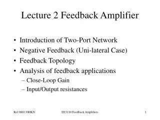
Learn about ideal and practical cases, gain analysis, g-parameters, loading effects, and examples for Shunt-Series Feedback Amplifiers. Explore midband gain, feedback factors, and input/output resistances with feedback in this comprehensive guide.

E N D
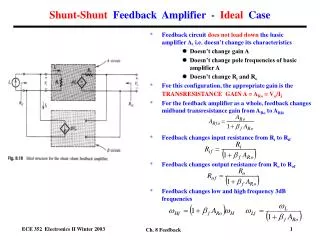
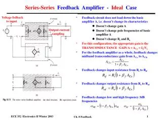
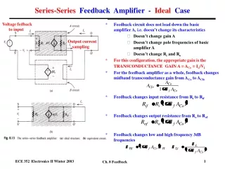
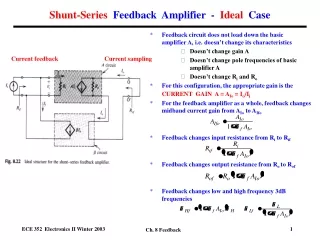
Shunt-Series Feedback Amplifier - Ideal Case • Feedback circuit does not load down the basic amplifier A, i.e. doesn’t change its characteristics • Doesn’t change gain A • Doesn’t change pole frequencies of basic amplifier A • Doesn’t change Ri and Ro • For this configuration, the appropriate gain is the CURRENT GAIN A = AIo = Io/Ii • For the feedback amplifier as a whole, feedback changes midband current gain from AIo to AIfo • Feedback changes input resistance from Ri to Rif • Feedback changes output resistance from Ro to Rof • Feedback changes low and high frequency 3dB frequencies Current feedback Current sampling Ch. 8 Feedback
Shunt-Series Feedback Amplifier - Ideal Case Gain Input Resistance Output Resistance Is=0 Io’ Vo’ Ch. 8 Feedback
Equivalent Network for Feedback Network • Feedback network is a two port network (input and output ports) • Can represent with g-parameter network (This is the best for this feedback amplifier configuration) • G-parameter equivalent network has FOUR parameters • G-parameters relate input and output currents and voltages • Two parameters chosen as independent variables. For G-parameter network, these are input voltages V1 and the output current I2 • Two equations relate other two quantities (input current I1 and output V2) to these independent variables • Knowing V1 and I2, can calculate I1 and V2 if you know the G-parameter values • G-parameters have various units of ohms, conductance (1/ohms=siemens) and no units ! Ch. 8 Feedback
Shunt-Series Feedback Amplifier - Practical Case • Feedback network consists of a set of resistors • These resistors have loading effects on the basic amplifier, i.e they change its characteristics, such as the gain • Can use g-parameter equivalent circuit for feedback network • Feedback factor f given by g12 since • Feedforward factor given by g21 (neglected) • g22gives feedback network loading on output • g11 gives feedback network loading on input • Can incorporate loading effects in a modified basic amplifier. Gain AIo becomes a new, modified gain AIo’. • Can then use analysis from ideal case I2 I1 g22 V2 V1 g11 g12I2 g21V1 Ch. 8 Feedback
Shunt-Series Feedback Amplifier - Practical Case • How do we determine the g-parameters for the feedback network? • For the input loading term g11 • We turn off the feedback signal by setting Io = I2 = 0. • We then evaluate the resistance seen looking into port 1 of the feedback network. • For the output loading term g22 • We short circuit the connection to the input so V1 = 0. • We find the resistance seen looking into port 2 of the feedback network. • To obtain the feedback factor f (also called g12 ) • We apply a test signal Io’ to port 2 of the feedback network and evaluate the feedback current If (also called I1 here) for V1 = 0. • Find f from f = If/Io’ I2 I1 g22 V2 g11 V1 g12I2 g21V1 Ch. 8 Feedback
Example - Shunt-Series Feedback Amplifier • Two stage [CE+CE] amplifier • Transistor parameters Given: =100, rx= 0 • Input and output coupling and emitter bypass capacitors, but direct coupling between stages • Capacitor in feedback connection removes Rf from DC bias • DC bias of two stages is coupled (bias of one affects the other) Ch. 8 Feedback
DC Bias Analysis VC1 VB2 (<<IC1 =870 A) (neglecting IB2 ) Ch. 8 Feedback
Example - Shunt-Series Feedback Amplifier • Redraw circuit to show • Feedback circuit • Type of output sampling (current in this case = Io) • Type of feedback signal to input (current in this case = If) Iout’ Iout’ Io’ Ch. 8 Feedback
Example - Shunt-Series Feedback Amplifier Iout’ Io’ Input Loading Effects Output Loading Effects Io’= 0 R1 R2 Ch. 8 Feedback
Example - Shunt-Series Feedback Amplifier Amplifier with Loading Effects but Without Feedback Ch. 8 Feedback
Example - Shunt-Series Feedback Amplifier Midband Gain Analysis Ri2 Iout’ IC’ Is Vi2 R1 R2 Ch. 8 Feedback
Midband Gain with Feedback • Determine the feedback factor f • Calculate gain with feedback AIfo • Note • f < 0and AIo < 0 • f AIo > 0 as necessary for negative feedback and dimensionless • f AIo is large so there is significant feedback. • Can change f and the amount of feedback by changing RF. • Gain is determined by feedback resistance + VE2 - Ch. 8 Feedback
Input and Output Resistances with Feedback • Determine input Ri and output Ro resistances with loading effects of feedback network. • Calculate input Rif and output Rof resistances for the complete feedback amplifier. Ro Ri Ch. 8 Feedback
Voltage Gain for Current Gain Feedback Amplifier • Can calculate voltage gain • Note - can’t calculate the voltage gain as follows: Ch. 8 Feedback
Equivalent Circuit for Shunt-Series Feedback Amplifier • Current gain amplifier A = Io/Is • Feedback modified gain, input and output resistances • Included loading effects of feedback network • Included feedback effects of feedback network • Significant feedback, i.e. f AIo is large and positive Rif AIfoI i Rof Ch. 8 Feedback
Frequency Analysis • Low frequency analysis of poles for feedback amplifier follows Gray-Searle (short circuit) technique as before. • Low frequency zeroes found as before. • Dominant pole used to find new low 3dB frequency. • For high frequency poles and zeroes, substitute hybrid-pi model with C and C(transistor’s capacitors). • Follow Gray-Searle (open circuit) technique to find poles • High frequency zeroes found as before. • Dominant pole used to find new high 3dB frequency. Ch. 8 Feedback
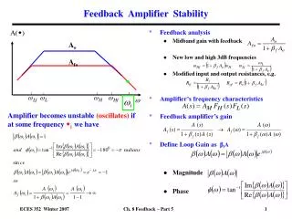
Summary of Feedback Amplifier Analysis • Identify the amplifier configuration by: • Output sampling • Io = series configuration • Vo = shunt configuration • Feedback to input • Io = shunt configuration • Vo = series configuration • Calculate loading effects of feedback network • On input • On output • Calculate appropriate midband gain A’ (modified by loading effects of feedback network) • Calculate feedback factor f. • Calculate midband gain with feedback Af. Xs Xi Xo Xf f • Calculate low frequency poles and zeroes. • Determine dominant (highest) • low frequency pole L including loading • effects of feedback network • Calculate new dominant low frequency • pole Lf . • Calculate high frequency poles and zeroes. • Determine dominant (lowest) • high frequency pole H including loading • effects of feedback network • Calculate new dominant high frequency • pole Hf . Ch. 8 Feedback
Summary of Feedback Amplifier Analysis Ch. 8 Feedback