Hierarchy
Hierarchy. Overview Background: Hierarchy surrounds us: what is it? Micro foundations of social stratification Ivan Chase: Structure from process Action --> Structure, not attributes Roger Gould A dyadic model of hierarchy formation David Krackhardt:


Hierarchy
E N D
Presentation Transcript
Hierarchy • Overview • Background: • Hierarchy surrounds us: what is it? • Micro foundations of social stratification • Ivan Chase: Structure from process • Action --> Structure, not attributes • Roger Gould • A dyadic model of hierarchy formation • David Krackhardt: • Deliberate Structure w. in organizations • Measures for the extent of hierarchy
Examples of Hierarchical Systems Linear Hierarchy (all triads transitive) Simple Hierarchy Branched Hierarchy Mixed Hierarchy
Examples of “Similar” Non-Hierarchical Systems Line Graph Acyclic Cycle
Chase’s Question: Where does hierarchy come from? Hierarchy surrounds us, in natural (animal and human) and controlled (laboratory, organizations) settings. How do we account for it? • Most previous research focuses on the static structure of hierarchy • Often consider the attributes of actors: strength, race, gender, education, size, etc.
Chase’s Question: Where does hierarchy come from? • The “Correlational Model” • Individual’s position in the hierarchy is due to their attributes (physical, social, etc.) • Mathematically, for the correlational model to be true, the correspondence between attributes and rank in the hierarchy would have to be extremely high (Pearson correlation of > .9). (See Chase, 1974 for details)
Chase’s Question: Where does hierarchy come from? • The “Pairwise interaction” model • Pairwise differences in each dyad account for position in the hierarchy. • “...it is assumed that each member of a group has a pairwise contest with each other member, that the winner of a contest dominates the loser in the group hierarchy, and that an individual has a particular probability of success in each contest.” • Model implies that there be one individual with a .95 probability of beating every other individual, another with a .95 probability of beating everyone but the most dominant, and so forth down the line. • The required conditions simply do not hold. As such, this explanation for where the hierarchy comes from cannot hold.
A B C D E Chase’s Question: Where does hierarchy come from? Chase focuses on the simple mathematical fact: Every linear hierarchy must contain all transitive triads. That is, the triad census for the network must have only 030T triads. Number of Type triads ---------------------- 1 - 003 0 ----------------------- 2 - 012 0 3 - 102 0 4 - 021D 0 5 - 021U 0 6 - 021C 0 7 - 111D 0 8 - 111U 0 9 - 030T 10 10 - 030C 0 11 - 201 0 12 - 120D 0 13 - 120U 0 14 - 120C 0 15 - 210 0 16 - 300 0 --------------------------- Sum (2 - 16): 10 What process could generate all 030T triads?
A A B C B C Transitive (030T) triad Intransitive (030C) triad Chase’s Question: Where does hierarchy come from? The elements: Dominance relations must by asymmetric, thus, the set of possible triads is limited.
Why Chase Finds Linear Hierarchy: Triad transitions (w/ Random Expectations) for Dominance Relations. P( 3 C) = .5*.5=.25 p=.5 030C p=.5 021C p=.5 p=1. P(030T)= (.5*.5 + .25*1 +.25*1) = .75 p=.25 003 012 030T p=1 021D p=.25 p=1 021U
Dominance Strategies That ensure a transitive hierarchy The “Double Attack” Strategy: The first attacker quickly attacks the bystander. This means we arrive at 21D, and any action on the part of the other two chickens will lead to a transitive triad. 003 012 030T 021D The “Double Receive” Strategy: The first attacker dominates B, and then the bystander quickly dominates B as well, leading to 21U, and any dominance between the first and second attacker will lead to a transitive triple. 003 012 030T 021U
030C 030C Dominance Strategies That may not lead to a transitive hierarchy “Attack the Attacker” The bystander attacks the first attacker. This could lead to a cyclic triad, and thus thwart hierarchy. 021C 003 012 030T 021C “Pass on the attack” The one who is attacked, attacks the bystander. Again, this could lead to a cycle, and thus thwart hierarchy. 003 012 030T
The evidence: 24 Chase Chicken Triads ( 0 stay) 1 ( 0 stay) 030C 1 021C 2 (1 stays) 1 23 (6 Fully Transitive) 17 012 003 (17 stay) 1 030 T 021D 4 4 Most Common Path Domination Reversal 021U New Domination ( 0 stay)
The Origins of Status Hierarchies: A formal model and empirical test Hierarchy & Inequality appear virtually universal. How do we account for it? • Two alternative explanations: • Individualist – that people vary in qualities that are locally salient • Structuralist – that differentiation results from the quality of social positions individuals occupy. • Third option: Hierarchy is explained as the product of an emergent social process without presupposing that the resulting assignment of actors to positions is a reflection of underlying qualities. The key is that: • “social hierarchies are understood to emerge and persists spontaneously rather than by conscious creation, but at the same time without ensuring that rewards exactly reflect differences in individual qualities” (p.1146)
The Origins of Status Hierarchies: A formal model and empirical test Theoretical claim: “the reason positions with greater and lesser advantage exist is that judgments about relative quality are socially influenced. Socially influenced judgments amplify underlying differences, so that actors who objectively rank above the mean on some abstract quality dimension are overvalued with those ranking below the mean are undervalued….Amplification occurs because observable interactions expressing judgments of quality are also cues to other actors seeking guidance for their own judgments.” (p.1147) Examples include the “Mathew effect” in science
The Origins of Status Hierarchies: A formal model and empirical test This claim is theoretically consistent with a Nash Equilibrium, in which everyone’s current choice of action is preferable to (or as good as) the alternatives so long as everyone else’s choice of action remains constant. IF attribution builds on others’ attributions, then, “the patterns should tend toward a stable state in which collective attributions confirm themselves in each time period.” The theory implies that “the only equilibria possible when there are absolutely no underlying differences across individuals are one in which everyone is ranked equally and one in which one actor receives attention while all others receive none.” (p.1149) This follows because of the ‘cascade’ effect of social influence.
The Origins of Status Hierarchies: A formal model and empirical test Since most observed structures fall between these two poles, something else must be going on as well. The mechanism employed rests on the returns to asymmetric admiration. “It is painful to pay attention to another person if the favor is not repaid. By the same token, it is particularly pleasant to receive attention when it is not solicited.” “Individuals should be less willing to demonstrate esteem toward those who do not return the favor and conversely may prefer to receive such demonstrations without reciprocating.”
The Origins of Status Hierarchies: A formal model and empirical test • The theory then makes three predictions: • Asymmetry in social relationships will be proportional to the difference in choice status (indegree) between pairs of actors. A high-status actor will be more weakly connected to any low-status actor that the latter is to her or him. This has to exceed the chance/tautology levels. • All else equal, pairs of actors who are similar in choice status will also be similar in the patterns of attachments they make to others. • Across all actors, the sum of attachments directed to others will be proportional to, but more evenly distributed than, the sum of attachments received.
The Origins of Status Hierarchies: A formal model and empirical test • Formally, the model: • Assumes a closed, finite population • The quantity of attachments varies across individuals • Each actor cares about: • The quality of each potential alter • The gap between their and the alter’s attachment to each other. Ui = utility for person i aij = attachment of person i to person j qj = quality of person j S = a weight of symmetry considerations relative to the quality of i’s alters in determining i’s welfare. In this model, q is determined exogenously
The Origins of Status Hierarchies: A formal model and empirical test To extend the model for social influence, assume that quality judgments are a function of peer influence: qij= i’s assessment of j’s quality Qj = exogenous quality of j W = relative weight of social influence on I’s judgment of j.
The Origins of Status Hierarchies: A formal model and empirical test Prediction from equation 6 (aggregate quality centered at 0)
The Origins of Status Hierarchies: A formal model and empirical test (Close-up of threshold region)
The Origins of Status Hierarchies: A formal model and empirical test Analysis of the model results is a set of testable propositions: • Asymmetry in attachments between any two actors is proportional to their differences in choice status • The relationship between choice status and asymmetry declines with group size • Any pair of actors i,j will be similar in the attachments they direct toward others in proportion as they are similar in choice status. • If sum(choice kj) – sum(choice ki) = 0, then aik – aij = 0. • Actors direct attachments to others in proportion to the quantity of attachments received • The slope of the function that transforms choice status into attachments directed outward is always less than unity. Consequently, the distribution of choice status (popularity) is more unequal than the distribution of out degree.
The Origins of Status Hierarchies: A formal model and empirical test .80
The Origins of Status Hierarchies: A formal model and empirical test
The Origins of Status Hierarchies: A formal model and empirical test So the model seems to be well supported by the data. -I’ve played a little with these models and Add Health, and they don’t perform as well, but the data don’t fit the assumptions either….
Graph Theoretic Dimensions of Informal Organizations What can SNA tell us about dominance in organizations? Krackhardt argues that an ‘Outree” is the archetype of hierarchy. • Krackhardt focuses on 4 dimensions: • 1) Connectedness • 2) Digraph hierarchic • 3) digraph efficiency • 4) least upper bound (what are the allowed triad types for an out-tree?)
Graph Theoretic Dimensions of Informal Organizations Connectedness: The digraph is connected if the underlying graph is a component. We can measure the extent of connectedness through reachability. Where V is the number of pairs that are not reachable, and N is the number of people in the network.
Reach: 1 2 3 4 5 1 0 1 2 1 0 2 1 0 1 2 0 3 2 1 0 3 0 4 1 2 3 0 0 5 0 0 0 0 0 Graph: 1 2 3 4 5 1 0 1 0 1 0 2 1 0 1 0 0 3 0 1 0 0 0 4 1 0 0 0 0 5 0 0 0 0 0 Digraph: 1 2 3 4 5 1 0 1 0 1 0 2 0 0 1 0 0 3 0 0 0 0 0 4 0 0 0 0 0 5 0 0 0 0 0 1 4 2 5 3 Graph Theoretic Dimensions of Informal Organizations How to calculate Connectedness: V = # of zeros in the upper diagonal of Reach: V = 4. C = 1 - [4/((5*4)/2)] = 1 - 4/1 = .6
Reachable: 1 2 3 4 5 1 0 1 1 1 0 2 1 0 1 1 0 3 1 1 0 1 0 4 1 1 1 0 0 5 0 0 0 0 0 Reach: 1 2 3 4 5 1 0 1 2 1 0 2 1 0 1 2 0 3 2 1 0 3 0 4 1 2 3 0 0 5 0 0 0 0 0 1 4 2 5 3 Graph Theoretic Dimensions of Informal Organizations How to calculate Connectedness: This is equivalent to the density of the reachability matrix. D = SR/(N(N-1)) = 12 /(5*4) = .6
Graph Theoretic Dimensions of Informal Organizations Graph Hierarchy: The extent to which people are asymmetrically reachable. Where V is the number of symmetrically reachable pairs in the network. Max(V) is the number of pairs where i can reach j or j can reach i.
1 4 2 5 3 Graph Theoretic Dimensions of Informal Organizations Graph Hierarchy: An example Dreachable 1 2 3 4 5 1 0 1 2 1 0 2 0 0 1 0 0 3 0 1 0 0 0 4 0 0 0 0 0 5 0 0 0 0 0 Digraph: 1 2 3 4 5 1 0 1 0 1 0 2 0 0 1 0 0 3 0 1 0 0 0 4 0 0 0 0 0 5 0 0 0 0 0 Dreach 1 2 3 4 5 1 0 1 2 1 0 2 0 0 1 0 0 3 0 1 0 0 0 4 0 0 0 0 0 5 0 0 0 0 0 V = 1 Max(V) = 4 H = 1/4 = .25
Graph Theoretic Dimensions of Informal Organizations Graph Efficiency: The extent to which there are extra lines in the graph, given the number of components. Where v is the number of excess links and max(v) is the maximum possible number of excess links
1 4 2 6 5 3 7 Graph Theoretic Dimensions of Informal Organizations Graph Efficiency: The minimum number of lines in a connected component is N-1 (assuming symmetry, only use the upper half of the adjacency matrix). In this example, the first component contains 4 nodes and thus the minimum required lines is 3. There are 4 lines, and thus V1= 4-3 = 1. The second component contains 3 nodes and thus minimum connectivity is = 2, there are 3 so V2 = 1. Summed over all components V=2. The maximum number of lines would occur if every node was connected to every other, and equals N(N-1)/2. For the first component Max(V1) = (6-3)=3. For the second, Max(V2) = (3-2)=1, so Max(V) = 4. Efficiency = (1- 2/4 ) = .5 1 2
Graph Theoretic Dimensions of Informal Organizations Graph Efficiency: Steps to calculate efficiency: a) identify all components in the graph b) for each component (i) do: i) calculate Vi = S(Gi)/2 - Ni-1; ii) calculate Max(Vi) = Ni(Ni-1) - (Ni-1) c) V = S(Vi), Max(V)= S(Max(Vi) d) efficiency = 1 - V/Max(V) Substantively, this must be a function of the average density of the components in the graph.
Graph Theoretic Dimensions of Informal Organizations Least Upper Boundedness: This condition looks at how many ‘roots’ there are in the tree. The LUB for any pair of actors is the closest person who can reach both of them. In a formal hierarchy, every pair should have at least one LUB. E In this case, E is the LUB for (A,D), B is the LUB for (F,G), H is the LUB for (D,C), etc. H B G C F A D
Graph Theoretic Dimensions of Informal Organizations Least Upper Boundedness: You get a violation of LUB if two people in the organization do not have an (eventual) common boss. Here, persons 4 and 7 do not have an LUB.
Distance matrix 1 2 3 4 5 6 7 8 9 1 1 1 1 2 2 2 2 1 1 1 3 1 1 4 1 5 1 6 1 1 1 2 7 1 1 8 1 9 1 Reachable matrix 1 2 3 4 5 6 7 8 9 1 1 1 1 1 1 1 2 1 1 1 3 1 1 4 1 5 1 6 1 1 1 1 7 1 1 8 1 9 1 Graph Theoretic Dimensions of Informal Organizations Least Upper Boundedness: Calculate LUB by looking at reachability. (Note that I set the diagonal = 1) A violation occurs whenever a pair is not reachable by at least one common node. We can get common reachability through matrix multiplication
Reachable matrix 1 2 3 4 5 6 7 8 9 1 1 1 1 1 1 1 2 1 1 1 3 1 1 4 1 5 1 6 1 1 1 1 7 1 1 8 1 9 1 Reachable Trans 1 2 3 4 5 6 7 8 9 1 1 2 1 1 3 1 1 4 1 1 1 5 1 1 1 6 1 7 1 1 8 1 1 9 1 1 1 1 1 Graph Theoretic Dimensions of Informal Organizations Least Upper Boundedness: Calculate LUB by looking at reachability. Common Reach 1 2 3 4 5 6 7 8 9 1 1 1 1 1 1 0 0 0 1 2 1 2 1 2 2 0 0 0 1 3 1 1 2 1 1 0 0 0 2 4 1 2 1 3 2 0 0 0 1 5 1 2 1 2 3 0 0 0 1 6 0 0 0 0 0 1 1 1 1 7 0 0 0 0 0 1 2 1 2 8 0 0 0 0 0 1 1 2 1 9 1 1 2 1 1 1 2 1 5 X = (R by S) (S by R) (R by R) Any place with a zero indicates a pair that does not have a LUB. R`*R = CR
Graph Theoretic Dimensions of Informal Organizations Least Upper Boundedness: Calculate LUB by looking at reachability. Where V = number of pairs that have no LUB, summed over all components, and:
Other characteristics of Hierarchy: • DAG: Directed, Acyclic, Graph • Graph that: • contains no cycles • at least one node has in-degree • Rank Cluster • Graph in which some number of nodes are mutually reachable, but asymmetrically reachable between groups. • Tree • A DAG with only one root • Centralization
Another method: Approximation based on permutation One characteristic of a hierarchy is that most of the ties fall on the upper triangle of the adjacency matrix. Thus, one way to get an order is by juggling the rows and columns until most of the ties are in the upper triangle. 1 1 1 1 1 1 1 1 1 1 2 3 4 5 6 7 8 9 1 2 3 4 5 6 7 8 1 1 2 1 3 4 1 1 5 1 6 1 1 7 8 1 1 1 9 1 1 1 1 1 11 1 12 1 1 13 1 1 1 14 1 1 1 15 16 17 1 18 1
13 1 1 1 14 1 1 1 9 1 1 1 1 1 2 1 11 1 5 1 1 1 8 1 1 1 18 1 17 1 4 1 1 6 1 1 12 1 1 3 7 15 16 Another method: Approximation based on permutation Re-ordered matrix