Multiple Alignment by profile HMM training and Phylogenetic Trees
500 likes | 653 Vues
Multiple Alignment by profile HMM training and Phylogenetic Trees. Elze de Groot & Anastacia Berdnikova. Topics. Multiple alignment with known HMM HMM training from unaligned sequences Avoiding local maxima Simulated annealing Noise injection Stochastic sampling traceback algorithm

Multiple Alignment by profile HMM training and Phylogenetic Trees
E N D
Presentation Transcript
Multiple Alignment by profile HMM trainingandPhylogenetic Trees Elze de Groot & Anastacia Berdnikova Elze de Groot & Anastasia Berdnikova
Topics • Multiple alignment with known HMM • HMM training from unaligned sequences • Avoiding local maxima • Simulated annealing • Noise injection • Stochastic sampling traceback algorithm • Model surgery • Phylogenetic trees Elze de Groot & Anastasia Berdnikova
Multiple alignment with known profile HMM • Multiple alignment and model known -> align large number of other family members • Calculating Viterbi alignment for every sequence • Residues in same match state are aligned in columns • That´s a difference between profile HMM and traditional multiple alignment Elze de Groot & Anastasia Berdnikova
Example • Model estimated from an alignment Elze de Groot & Anastasia Berdnikova
Example continued • The most probable paths and alignment Elze de Groot & Anastasia Berdnikova
Profile HMM training from unaligned sequences • Algorithm: Elze de Groot & Anastasia Berdnikova
Initial Model • Choose length of model - M is number of match states - set M to be the average length • Choose initial models carefully • Randomness in choice of initial model Elze de Groot & Anastasia Berdnikova
Parameter Estimation • Use forward and backward variables to re-estimate emission and transition probability parameters • Baum-Welch re-estimation can be replaced by viterbi alternative Elze de Groot & Anastasia Berdnikova
Forward Algorithm Elze de Groot & Anastasia Berdnikova
Backward algorithm Elze de Groot & Anastasia Berdnikova
Baum-Welch re-estimation equations • Expected emission counts from sequence x Elze de Groot & Anastasia Berdnikova
Baum-Welch re-estimation equations • Expected transition counts from sequence x Elze de Groot & Anastasia Berdnikova
Avoiding local maxima • Baum-Welch guaranteed to find local maxima • Not guaranteed it is anywhere near global optimum or biologically reasonable solution • Reason: models are long -> many options to get wrong solution Elze de Groot & Anastasia Berdnikova
Avoiding local maxima • Use stochastic search algorithm • Commonly used: Simulated annealing Elze de Groot & Anastasia Berdnikova
Simulated annealing • Some compounds only cristallise if they are slowly annealed from high to low temperature • Optimisation problem: minimise function ´energy´ E(x) • Maximising function same as minimising negative value of function Elze de Groot & Anastasia Berdnikova
Simulated annealing (2) • ´temperature´ T • Probability of ´state´ x is given by Gibbs distribution • Partition function: • x usually multidimensional so impossible to calculate Z Elze de Groot & Anastasia Berdnikova
Simulated annealing (3) • T0, all configurations except with lowest energy are prob 0 (system is ´frozen´) • T, All configuration have same prob (system is ´molten´) • With crystallisation: minimum can be found by sampling this distribution at high temperature first and then decreasing temperatures Elze de Groot & Anastasia Berdnikova
Simulated annealing for HMM • Natural energy function negative log of likelihood –logP(data|) • Non-trivial, the two methods I´m going to mention are approximations Elze de Groot & Anastasia Berdnikova
Noise injection • Adding noise to counts estimated in forward-backward procedure and let size of noise decrease slowly • In Krogh et al.[1994] the noise was generated by a random walk in the initial model Elze de Groot & Anastasia Berdnikova
Simulated annealing Viterbi estimation • If there are N sequences, there´s an exact translation from the N paths 1,…, N to the parameters of the model • Treat the paths as fundamental parameters in which to maximise the likelihood • Simulated annealing done in these variables instead of the model parameters Elze de Groot & Anastasia Berdnikova
Simulated annealing Viterbi estimation • Denominator is Z, the partition function -> sum over all paths • Can be obtained by modified forward algorithm using exponentiated transmission and emission parameters Elze de Groot & Anastasia Berdnikova
Simulated annealing Viterbi estimation • Exponentiated transmission parameter • âij = aij1/T • Exponentiated emission parameter • êj(x) = ej(x)1/T • Used in place of unmodified probability parameters in forward algorithm • Z is result of forward algorithm Elze de Groot & Anastasia Berdnikova
Simulated annealing Viterbi estimation • Algorithm: Stochastic sampling traceback algorithm for HMMs Initialisation: πL+1 = End. Recursion: for L+1 ≥ i ≥ 1, Elze de Groot & Anastasia Berdnikova
Simulated annealing Viterbi vs Viterbi • Key difference: • Viterbi selects highest probable path for each sequence • Simulated annealing samples each path according to the likelihood of the path Elze de Groot & Anastasia Berdnikova
Model Surgery • During training a model two things can happen: • (a) some match states are redundant and should be absorbed in insert state • (b) one or more insert states aborb too much sequence, in which case they should be expanded Elze de Groot & Anastasia Berdnikova
Model Surgery • How much is a certain transition used by training sequences • Usage of match state is sum of counts for all letters in state Elze de Groot & Anastasia Berdnikova
Model surgery • If match state is used by less than ½ sequences -> delete module • If more than ½ of sequences use the transitions into an insert state, this is expanded to new modules Elze de Groot & Anastasia Berdnikova
Model surgery – Example SAM • I tried a sequence in SAM with and without model surgery • Same 7 sequences as in example before • Parameters <cutinsert 0.25> <cutmatch 0.5> -> delete any match state used by fewer than half the sequences, and insert match states for any insert node used by greater than one quarter of the sequences Elze de Groot & Anastasia Berdnikova
Without model surgery >seq1 FPHFD.....L...S.....-HGSAQ >seq2 FESFG.....D...LstpdaVMGNPK >seq3 FDRFKhlkteA...E.....MKASED >seq4 FTQFA.....G...Kdles.IKGTAP >seq5 FPKFK.....G...LttadqLKKSAD >seq6 FSFLK.....GtseV.....PQNNPE >seq7 FGFSG.....A...-.....--SDPG With model surgery >seq1 FPHF.DLS-..-..--HGSAQ >seq2 FESF.GDLStpD..AVMGNPK >seq3 FDRF.KHLK..TeaEMKASED >seq4 FTQFaGKDL..E..SIKGTAP >seq5 FPKF.KGLTtaD..QLKKSAD >seq6 FSFL.KGTS..E..VPQNNPE >seq7 FGFS.G---..-..--ASDPG Model surgery – Example SAM Elze de Groot & Anastasia Berdnikova
Building phylogenetic trees Elze de Groot & Anastasia Berdnikova
Overview • The tree of life – description • Background on trees Elze de Groot & Anastasia Berdnikova
Multiple alignment and trees • Alignment of sequences should take account of their evolutionary relationship. [Sankoff, Morel & Cedergren, 1973] • Several progressive alignment algorithms use a ‘guide tree’ (to guide the clustering process). • We begin to build trees. Elze de Groot & Anastasia Berdnikova
The tree of life • The similarity of molecular mechanisms of the organisms that have been studied strongly suggests that all organisms on Earth had a common ancestor. Thus any sets of species is related, and this relationship is called a phylogeny. • Usually therelationship can be represented by a phylogenetic tree. Elze de Groot & Anastasia Berdnikova
Zuckerkandl & Pauling’s paper [1962] showed that molecular sequences provide sets of morphological characters that can carry a large amount of information. • An assumption: the sequencies we want to analyze on thephylogeny matter have descended from some common ancestral gene in a common ancestral species. • Gene duplication exists => we have to check the assumption carefully. Elze de Groot & Anastasia Berdnikova
Gene duplication and speciation • By another mechanism, gene duplication, two sequences can also be separated and diverge from the common ancestor. • Genes which diverged because of speciationare called orthologues. Genes which diverged by gene duplication are called paralogues. Elze de Groot & Anastasia Berdnikova
A tree of orthologues: alpha haemoglobins HBA_ACCGE, HBA_AEGMO, HBA_AILFU, HBA_AILME, HBA_ALCAA, HBA_ALLMI, HBA_AMBME, HBA_ANAPL (SWISS-PROT). Elze de Groot & Anastasia Berdnikova
A tree of paralogues: HBAT_HUMAN, HBAZ_HUMAN, HBA_HUMAN, HBB_HUMAN, HBD_HUMAN, HBE_HUMAN, HBG_HUMAN, MYG_HUMAN (SWISS-PROT). Elze de Groot & Anastasia Berdnikova
Background on trees • All trees will be assumed to be binary (an edge that branches splits into two daughter edges). • Each edge ofthe tree has a certain amount of evolutionary divergence associated to it. We adopt the general term ‘length’, which will be represented by lengthes of edges on figures. • A true biological phylogeny has a ‘root’, or ultimate ancestor of all sequences. Elze de Groot & Anastasia Berdnikova
Rooted and unrooted tree Elze de Groot & Anastasia Berdnikova
A tree with a given labelling will be called a labelled branching pattern. • We refer to this as the tree topology and denote it by T. • Lengths of the edges: ti with a suitable numbering scheme for the is. Elze de Groot & Anastasia Berdnikova
Counting and labelling Rooted tree: • n leaves, plus (n-1) branchnodes in addition to leaves -> we have 2n-1 nodes in all, and 2n-2 edges. • leaves – 1..n, branch nodes – n+1 .. 2n-1, (2n-1)th node is root. Elze de Groot & Anastasia Berdnikova
Counting and labelling Unrooted tree: • n leaves, 2n-2 nodes and 2n-3 edges. • a root can be added at any of its edges => we can get 2n-3 rooted trees. Elze de Groot & Anastasia Berdnikova
Number of rooted and unrooted trees A root can be added at any edge, producing 2n-3 rooted trees from unrooted tree => there are (2n-3) times as many rooted trees as unrooted trees, for a given number n of leaves. Elze de Groot & Anastasia Berdnikova
Instead of the root, we can add an extra edge or ‘branch’ with a distinct label in its leaf. Elze de Groot & Anastasia Berdnikova
There are three such trees with (2n-3)=5 leaves – they are distinct labelled branching patterns. • There are then five ways of adding a further branch labelled with a distinct label (‘5’), giving in all 3x5=15 unrooted trees with five leaves. • The number of unrooted trees with n leaves is equal to 3*5*...*(2n-5) = (2n-5)!! So, we have (2n-3)!! rooted trees with n leaves. Elze de Groot & Anastasia Berdnikova
Building phylogenetic trees Questions? Elze de Groot & Anastasia Berdnikova
Exercise 7.2 • The trees with three and four leaves in Figure 7.3 all have the same unlabelled branching pattern. For both rooted and unrooted trees, how many leaves do there have to be to obtain more than one unlabelled branching pattern? Find a recurrence relation for the number of rooted trees. (Hint: consider the trees formed by joining two trees at their root). Elze de Groot & Anastasia Berdnikova
Exercise 7.2 Elze de Groot & Anastasia Berdnikova
Exercise 7.3 • All trees considered so far have been binary, but one can envisage ternary trees that, in their rooted form, have three branches descending from a branch node. If there are m branch nodes in an unrooted ternary tree, how many leaves are there and how many edges? Elze de Groot & Anastasia Berdnikova
Exercise 7.4 • Consider next a composite unrooted tree with m ternary branch nodes and n binary branch nodes. How many leaves are there, and how many edges? Let Nm,ndenote the number of distinct labelled branching patterns of this tree. Extend the counting argument for binary trees to show that Nm,n = (3m+2n-1)N m,n-1 + (n+1)N m-1,n+1 (Hint: the first term after the ‘=’ counts the number of ways that a new edge can be added to an existing edge, thereby creating an additional binary node; the second term corresponds to edges added at binary nodes, thereby producing ternary nodes.) Elze de Groot & Anastasia Berdnikova
