Download
1 / 47
470 likes | 1.03k Vues
The Examination of Residuals. Introduction. Much can be learned by examinging residuals. . This is true not only for linear regression models, but also for nonlinear regression models and analysis of variance models. .

E N D
Introduction • Much can be learned by examinging residuals. • This is true not only for linear regression models, but also for nonlinear regression models and analysis of variance models. • In fact, this is true for any situation where a model is fitted and measures of unexplained variation (in the form of a set of residuals) are available for examination.
Quite often models that are proposed initially for a set of data are incorrect to some extent. • An important part of the modeling process is diagnosing the flaws in these models. • Much of this can be done by carefully examining the residuals
where is an observation and is the corresponding fitted value obtained by use of the fitted model. • The residuals are defined as the n differences :
the residuals should exhibit tendencies that tend to confirm the above assumptions, or at least, should not exhibit a denial of the assumptions. If the fitted model is correct, The behaviour of the residuals should reflect to some extent the assumptions made regarding the random noise component the residuals are “estimators” of the random noise component of the model
After examination of the residuals we shall be able to conclude either: (1) the assumptions appear to be violated (in a way that can be specified), or (2) the assumptions do not appear to be violated.
The methods for examining the residuals are: • sometimes graphical and • sometimes statistical
The the assumptions usually made regarding the error term in regression models are • Mean zero. • Common variance (standard deviation) (Homogeneity of variance) • Independence (uncorrelated) • Normal distribution
If the residuals contradict these assumptions than the model may be incorrect. Either because • The random error term does not satisfy some of the assumptions • Common variance (standard deviation) (Homogeneity of variance) • Independence (uncorrelated) • Normal distribution • Or • The model is incorrect (indicated by non-zero mean residuals )
1. Overall. The principal ways of plotting the residuals ei are: 2. In time sequence, if the order is known. 3. Against the fitted values 4. Against the independent variables xij for each value of j
Overall Plot The residuals can be plotted in an overall plot in several ways.
5. a normal plot or a half normal plot on standard probability paper.
Does our overall plot contradict this idea? If our model is correct these residuals should (approximately) resemble observations from a normal distribution with zero mean. • Does the plot exhibit appear abnormal for a sample of n observations from a normal distribution. • How can we tell? • With a little practice one can develop an excellent "feel" of how abnormal a plot should look before it can be said to appear to contradict the normality assumption.
1. The Kolmogorov-Smirnov test. • The standard statistical test for testing Normality are: 2. The Chi-square goodness of fit test
The Kolmogorov-Smirnov uses the empirical cumulative distribution function as a tool for testing the goodness of fit of a distribution. The Kolmogorov-Smirnov test • The empirical distribution function is defined below for n random observations Fn(x) = the proportion of observations in the sample that are less than or equal to x.
Let F0(x) denote the hypothesized cumulative distribution function of the population (Normal population if we were testing normality) If F0(x) truly represented distribution of observations in the population than Fn(x) will be close to F0(x) for all values of x.
Fn(x) F0(x)
The Kolmogorov-Smirinov test statistic is : = the maximum distance between Fn(x) and F0(x). • If F0(x) does not provide a good fit to the distributions of the observation - Dn will be large. • Critical values for are given in many texts and computed by most programs
The Chi-square test uses the histogram as a tool for testing the goodness of fit of a distribution. The Chi-square goodness of fit test • Let fi denote the observed frequency in each of the class intervals of the histogram. • Let Ei denote the expected number of observation in each class interval assuming the hypothesized distribution.
The hypothesized distribution is rejected if the statistic: • is large. (greater than the critical value from the chi-square distribution with m - 1 degrees of freedom. • m = the number of class intervals used for constructing the histogram).
The in the above tests it is assumed that the residuals are independent with a common variance of s2. Note. This is not completely accurate for this reason: Although the theoretical random errors ei are all assumed to be independent with the same variance s2, the residuals are not independent and they also do not have the same variance.
They will however be approximately independent with common variance if the sample size is large relative to the number of parameters in the model. It is important to keep this in mind when judging residuals when the number of observations is close to the number of parameters in the model.
The residuals should exhibit a pattern of independence. Time Sequence Plot If the data was collected in time there could be a strong possibility that the random departures from the model are autocorrelated.
Namely the random departures for observations that were taken at neighbouring points in time are autocorrelated. This autocorrelation can sometimes be seen in a time sequence plot. The following three graphs show a sequence of residuals that are respectively i) positively autocorrelated , ii) independent and iii) negatively autocorrelated.
There are several statistics and statistical tests that can also pick out autocorrelation amongst the residuals. The most common are: i) The Durbin Watson statistic ii) The autocorrelation function iii) The runs test
The Durbin-Watson statistic which is used frequently to detect serial correlation is defined by the following formula: The Durbin Watson statistic: If the residuals are serially correlated the differences, ei - ei+1, will be stochastically small. Hence a small value of the Durbin-Watson statistic will indicate positive autocorrelation. Large values of the Durbin-Watson statistic on the other hand will indicate negative autocorrelation. Critical values for this statistic, can be found in many statistical textbooks.
The autocorrelation function at lag k is defined by: The autocorrelation function: This statistic measures the correlation between residuals the occur a distance k apart in time. One would expect that residuals that are close in time are more correlated than residuals that are separated by a greater distance in time. If the residuals are independent than rk should be close to zero for all values of k A plot of rk versus k can be very revealing with respect to the independence of the residuals. Some typical patterns of the autocorrelation function are given below:
This statistic measures the correlation between residuals the occur a distance k apart in time. One would expect that residuals that are close in time are more correlated than residuals that are separated by a greater distance in time. If the residuals are independent than rk should be close to zero for all values of k A plot of rk versus k can be very revealing with respect to the independence of the residuals.
Auto correlation pattern for independent residuals Some typical patterns of the autocorrelation function are given below:
Various Autocorrelation patterns for serially correlated residuals
This test uses the fact that the residuals will oscillate about zero at a “normal” rate if the random departures are independent. The runs test: If the residuals oscillate slowly about zero, this is an indication that there is a positive autocorrelation amongst the residuals. If the residuals oscillate at a frequent rate about zero, this is an indication that there is a negative autocorrelation amongst the residuals.
+ + + - - + + - - - + + + In the “runs test”, one observes the time sequence of the “sign” of the residuals: and counts the number of runs (i.e. the number of periods that the residuals keep the same sign). This should be low if the residuals are positively correlated and high if negatively correlated.
Other Graphical Plots Residuals versus fitted values Residuals vs predictor variables
If we "step back" from this diagram and the residuals behave in a manner consistent with the assumptions of the model we obtain the impression of a horizontal "band " of residuals which can be represented by the diagram below. Plot Against fitted values and the Predictor Variables Xij
Outliers An outlier is an observation that is not following the normal pattern of the other observations. Individual observations lying considerably outside of this band indicate that the observation may be and outlier. Such an observation can have a considerable effect on the estimation of the parameters of a model. Sometimes the outlier has occurred because of a typographical error. If this is the case and it is detected than a correction can be made. If the outlier occurs for other (and more natural) reasons it may be appropriate to construct a model that incorporates the occurrence of outliers.
If our "step back" view of the residuals resembled any of those shown below we should conclude that assumptions about the model are incorrect. Each pattern may indicate that a different assumption may have to be made to explain the “abnormal” residual pattern. b) a)
Pattern a) indicates that the variance the random departures is not constant (homogeneous) but increases as the value along the horizontal axis increases (time, or one of the independent variables). This indicates that a weighted least squares analysis should be used. The second pattern, b) indicates that the mean value of the residuals is not zero. This is usually because the model (linear or non linear) has not been correctly specified. Linear and quadratic terms have been omitted that should have been included in the model.
Example = Motor Vehicles • Dependent variable – Mileage (mpg) • Independent variables • Weight • Horsepower • Engine Size
First Step • Fit a Linear Model using Stepwise linear regression • With only 3 independent variables we could also consider all possible subsets regression. We need to use Minitab for this procedure