Download
1 / 50
510 likes | 623 Vues
Explore the use of residuals in regression analysis to identify patterns and outliers. Learn how to interpret residual plots to detect issues in the analysis. Understand the steps to compute residuals and their significance in evaluating data points.

E N D
Residuals A continuation ofregression analysis
Lesson Objectives • Continue to build on regression analysis. • Learn how residual plotshelp identify problems with the analysis.
CaseXY 1 73 175 2 68 158 3 67 140 4 72 207 5 62 115 ^ Wt = – 332.73 + 7.189 Ht Example 1: Sample of n = 5 students,Y = Weight in pounds,X = Height in inches. continued … Prediction equation: To be foundlater. r-square = ? Std. error = ?
^ Y = – 332.7 + 7.189X Example 1, continued 220 · 200 · 180 · 160 WEIGHT Residuals = distance from point to line, measuredparallel to Y- axis. · 140 · 120 100 60 64 68 72 76 HEIGHT
Calculation: For each case, residual = observed value estimated mean ^ ei = yi - yi For the ith case,
Compute the fitted value and residual for the 4th person in the sample; i.e., X = 72 inches, Y = 207 lbs. ^ y = fitted value = 4 ^ y4 - y4 Example 1, continued -332.73 + 7.189() = _________ residual = e4 = = = __________
ResidualPlots Scatterplot of residuals vs. the predicted means of Y, Y; or an X-variable. ^
^ Y = – 332.7 + 7.189X Example 1, continued e4 = +22.12. 220 · 200 · 180 · 160 WEIGHT Residuals = distance from point to line, measuredparallel to Y- axis. · 140 · 120 100 60 64 68 72 76 HEIGHT
Example 1, continued · 24 e4 is theresidual for the 4th case,= +22.12. Residual Plot 16 8 · · 0 Residuals · -8 Regression line from previous plot is rotated to horizontal. · -16 -24 60 64 68 72 76 HEIGHT
Residual Plot Scatterplot of residuals versus the predicted means of Y, Y; or an X-variable, or Time. ^ Expect random dispersion around a horizontal line at zero. Problems occur if: • Unusual patterns • Unusual cases
Residuals versus X l l l l l l l l l l l Residuals l 0 l l l l l l l l l Good random pattern X, or time
Residuals versus X l l l l l l l l l l l l l Residuals l l l 0 l l l l l l l Next step: ________ to determineif a recording error has occurred. l Outliers? X, or time
Residuals versus X Next step: Add a “quadratic term,”or use “______.” l l l l l l l l l l l l Residuals l l 0 l l l l l l l l l l l l l l Nonlinear relationship X, or time
Residuals versus X l Next step: Stabilize variance by using “________.” l l l l l l l l l l l l l l l l Residuals l 0 l l l l l l l l l l l l l l l l l l l l Variance is increasing X, or time
Unusual patterns: qPossible curvature in the data. qVariances that are not constant as X changes. Unusual cases: qOutliers q High leverage cases q Influential cases Residual Plots help identify
Three properties of Residuals illustrated with somecomputations.
73 175 68 158 67 140 72 207 62 115 ^ ^ e = Y – Y Y .01 Property 1. Y = Weight X = Height ^ Y = – 332.73 + 7.189 X Residuals XY –17.07 192.07 Find the sum of the residuals. 156.12 1.88 . . . round-off error
1. Residuals always sum to zero. Properties of Least Squares Line Sei = 0.
73 175 68 158 67 140 72 207 62 115 ^ ^ e = Y – Y Y 867.98 .01 Property 2. Y = Weight X = Height ^ Y = – 332.73 + 7.189 X e2 XY 192.07 156.12 148.93184.88112.99 –17.07 1.88 –8.93 22.12 2.01 291.38 3.53 79.74489.29 4.04 Find the sum of squaresof the residuals.
1.Residuals always sum to zero. “SSE for any other line”. Sei2= SSE = 867.98 < Properties of Least Squares Line 2. This “least squares” line produces a smaller “Sum of squared residuals” than any other straight line can.
X = 68.4, Y = 159 Y Property 3. 220 · 200 · 180 · 160 WEIGHT · 140 · 120 100 60 64 68 72 76 X HEIGHT
1. Residuals always sum to zero. 2. This “least squares” line produces a smaller “Sum of squared residuals” than any other straight line can. 3. Line always passes through the point ( x, y ). Properties of Least Squares Line
Illustration of unusual cases: • Outliers • Leverage • Influential
X Y outlier l l l l l l “Unusual point” does not follow pattern. It’s near the X-mean; the entire line pulled toward it. l l l l l l l l l l X
X l Y l “Unusual point” does not follow pattern. The line is pulled down and twistedslightly. l l l l l l l l l l l outlier l l l X
X “Unusual point” is farfrom the X-mean, but still follows the pattern. Y l Highleverage l l l l l l l l l l l l l l X
influential X “Unusual point” is far from the X-mean, but does not follow the pattern.Line really twists! Y l l l l l l l l l l l l l l l l leverage & outlier, X
High Leverage Case: An extreme X value relative to the other X values. Definitions: Outlier: An unusual y-value relative to the pattern of the other cases.Usually has a large residual.
has an unusually largeeffecton the slope of the least squares line. Definitions: continued Influential Case
High leverage Definitions: continued Conclusion: potentially influential. High leverage & Outlier influential!!
The least squares regression line is not resistantto unusual cases. Why do we care about identifying unusual cases?
Lesson Objectives • Learn two ways to use Minitab to runa regression analysis. • Learn how to read output from Minitab.
Example 3, continued … Can height be predicted using shoe size? Step 1? DTDP
Female Male Example 3, continued … Can height be predicted using shoe size? Graph Scatterplot Plot … “Jitter” added in X-direction. The scatter for eachsubpopulation is about the same; i.e., there is“constant variance.”
Example 3, continued … Stat Method 1 Regression Regression … Y = a + bX
Example 3, continued … Copied from “Session Window.” Can height be predicted using shoe size? Regression Analysis: Height versus Shoe Size The regression equation is Height = 50.5 + 1.87 Shoe Size Predictor Coef SE Coef T P Constant 50.5230 0.5912 85.45 0.000 Shoe Siz 1.87241 0.06033 31.04 0.000 S = 1.947 R-Sq = 79.1% R-Sq(adj) = 79.0% Analysis of Variance Source DF SS MS F P Regression 1 3650.0 3650.0 963.26 0.000 Error 255 966.3 3.8 Total 256 4616.3
Least squares estimated coefficients. Example 3, continued … Can height be predicted using shoe size? Regression Analysis: Height versus Shoe Size The regression equation is Height = 50.5 + 1.87 Shoe Size Predictor Coef SE Coef T P Constant 50.5230 0.5912 85.45 0.000 Shoe Siz 1.87241 0.06033 31.04 0.000 S = 1.947 R-Sq = 79.1% R-Sq(adj) = 79.0% Analysis of Variance Source DF SS MS F P Regression 1 3650.0 3650.0 963.26 0.000 Error 255 966.3 3.8 Total 256 4616.3 Total “Degrees of Freedom”= Number of cases - 1
SSRTSS 3650.04616.3 R-Sq = = Example 3, continued … Can height be predicted using shoe size? Regression Analysis: Height versus Shoe Size The regression equation is Height = 50.5 + 1.87 Shoe Size Predictor Coef SE Coef T P Constant 50.5230 0.5912 85.45 0.000 Shoe Siz 1.87241 0.06033 31.04 0.000 S = 1.947 R-Sq = 79.1% R-Sq(adj) = 79.0% Analysis of Variance Source DF SS MS F P Regression 1 3650.0 3650.0 963.26 0.000 Error 255 966.3 3.8 Total 256 4616.3
3.8 S = MSE = Example 3, continued … Can height be predicted using shoe size? Regression Analysis: Height versus Shoe Size The regression equation is Height = 50.5 + 1.87 Shoe Size Predictor Coef SE Coef T P Constant 50.5230 0.5912 85.45 0.000 Shoe Siz 1.87241 0.06033 31.04 0.000 S = 1.947 R-Sq = 79.1% R-Sq(adj) = 79.0% Analysis of Variance Source DF SS MS F P Regression 1 3650.0 3650.0 963.26 0.000 Error 255 966.3 3.8 Total 256 4616.3 Standard Error of Regression.Measure of variation around the regression line. Sum of squared residuals Mean Squared ErrorMSE
Example 3, continued … Can height be predicted using shoe size? Are there anyproblems visiblein this plot? ___________ No “Jitter” added.
Height = 50.52 + 1.872 Shoe Example 3, continued … Can height be predicted using shoe size? Least squares regression equation: Std. error = 1.947 inches r-square = 79.1%, The two summary measuresthat should always begiven with the equation.
Example 3, continued … Can height be predicted using shoe size? Stat Method 2 This program gives a scatterplot with the regression superimposed on it. Regression Fitted Line Plot … Y = a + bX
Example 3, continued … Can height be predicted using shoe size? The fit looks
Example 3, continued … Can height be predicted using shoe size? Regression Analysis: Height versus Shoe Size The regression equation is Height = 50.5 + 1.87 Shoe Size Predictor Coef SE Coef T P Constant 50.5230 0.5912 85.45 0.000 Shoe Siz 1.87241 0.06033 31.04 0.000 S = 1.947 R-Sq = 79.1% R-Sq(adj) = 79.0% Analysis of Variance Source DF SS MS F P Regression 1 3650.0 3650.0 963.26 0.000 Error 255 966.3 3.8 Total 256 4616.3 What information do these values provide?
1 How do you determine if theX-variable is a useful predictor? Use the“t-statistic”or the F-stat. “t” measures how many standard errors the estimated coefficient is from “zero.” “F” = t2 for simple regression.
2 How do you determine if theX-variable is a useful predictor? A “P-value” is associated with “t” and “F”. The further “t” and “F” are from zero,in either direction, the smaller the corresponding P-value will be. P-value: a measure of the “likelihoodthat the true coefficient IS ZERO.”
If the P-value IS SMALL (typically “<0.10”), 3 then conclude: 1. It is unlikely that the true coefficient is really zero, and therefore, 2. The X variable IS a useful predictor for the Y variable. Keep the variable! If the P-value is NOT SMALL (i.e., “> 0.10”), then conclude: 1. For all practical purposes the true coefficient MAY BE ZERO; therefore 2. The X variable IS NOT a useful predictor of the Y variable. Don’t use it.
Example 3, continued … Can height be predicted using shoe size? Could “shoe size”have a truecoefficient thatis actually “zero”? Regression Analysis: Height versus Shoe Size The regression equation is Height = 50.5 + 1.87 Shoe Size Predictor Coef SE Coef T P Constant 50.5230 0.5912 85.45 0.000 Shoe Siz 1.87241 0.06033 31.04 0.000 S = 1.947 R-Sq = 79.1% R-Sq(adj) = 79.0% Analysis of Variance Source DF SS MS F P Regression 1 3650.0 3650.0 963.26 0.000 Error 255 966.3 3.8 Total 256 4616.3 “t” measures how many standard errors the estimated coefficient is from “zero.” P-value: a measure of the likelihoodthat the true coefficient is “zero.” The P-value for Shoe Size IS SMALL (< 0.10). Conclusion: The “shoe size” coefficient is NOT zero!“Shoe size” IS a useful predictor of the mean of “height”.
The logic just explained is statistical inference. This will be covered in more detail during the last three weeks of the course.