Download
1 / 39
420 likes | 625 Vues
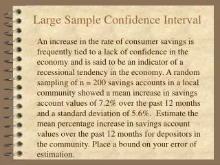
Lecture 9. Law of large numbers. Central limit theorem. Confidence interval. Hypothesis testing. Types of errors. Some practice with the Normal distribution (please open Lect9_ClassPractice). 1. Math aptitude scores are distributed as N(500,100).

E N D
Lecture 9. • Law of large numbers. • Central limit theorem. • Confidence interval. • Hypothesis testing. Types of errors.
Some practice with the Normal distribution (please open Lect9_ClassPractice) 1. Math aptitude scores are distributed as N(500,100). Find: a. the probability that the individual score exceeds 600 andb. the probability that the individual score exceeds 600 given that it exceeds 500 2. What mathematics SAT score, can be expect to occur with the probability 0.90 or greater ?
The (weak) law of large numbers (The following result is also known as a Bernoulli theorem). Let X1 , X2 ..., Xn be a sequence of independent and identically distributed (iid) random variables, each having a mean EXi = and standard deviation Define a new variable, the “sample mean” One should keep in mind that isalso a random variable : it randomly changes between different samples of the same size n, and those changes are sensitive to the size of the sample, n: Example (Lect9_LargeNumbers.nb).
Using the properties of expectations it is easy to prove that Using the properties of the variances (see Lect. 8) we can also prove that Then, using the Chebyshev’ inequality, (we use it without prove) one can find
where is any (but typically small) positive number. Let us discuss this result. The left side contains the probability that the deviation between the sample average, and the mean value of the individual random variable,, exceeds . The right hand side shows that this probability decreases as 1/n for large n. Thus, one can say that “ converges to in probability”. (Weak) Law of Large Numbers.Suppose X1 ,X2 ...,Xn are i.i.d. with finite E(Xi) =. Then, as (9.5), converges to in probability.
(9.5) could be called the fundamental theorem of statistics because it says that the sample mean is close to the mean of the underlying population when the sample is large. It implies that we do not have to measure the weights of all American 30 year old males in order to find their average weight.We can use the weights of 1000 individuals chosen at random. Later on we will discuss how close the mean on the sample of this size will be to the mean of the underlying population.
Experiments with dice and coins show that the rate of convergence to the average value is quite slow. Using (9.4) we can understand why it is so. Suppose that we flip a coin n = 1000 times and let Xibe 1 if the i-th toss is Heads and 0 otherwise. The Xi are Bernoulli random variables with p=P(Xi=1)=0.5. Exi=p=0.5. VarXi = (1-p)2p+ p2(1-p)=(1-p)p(1-p+p)=p(1-p)=1/4. Taking =0.05 (which is the 10 % of the expected value), we find: We can see that the probability of a comparatively large fluctuation (10 % of the mean value) is not too small. It explains the large irregularities that we can find in the pictures.
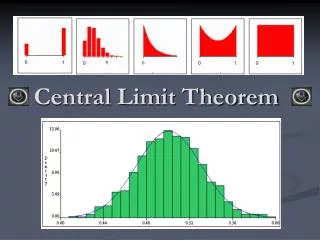
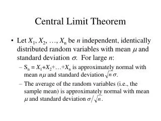
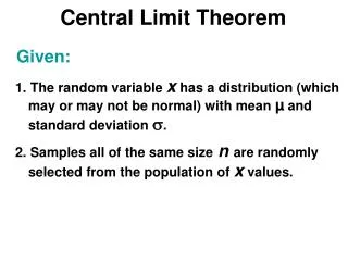
Central Limit Theorem. The Law of Large Numbers indicated that the sample average converges in probability to the population average. Now our concern are the probability distributions. Suppose that we know a distribution for i.i.d. Xi. We wonder how the distribution of the sum of Xi is related to the individual distributions. Reiteration: assuming we know pdf(Xi), what can we tell about the pdf( ) for large n. Central Limit Theorem(First formulation)Suppose X1 ,X2 ...,Xn are i.i.d. with E(Xi)= andfiniteVar(Xi)= 2. Then, as (9.5) where denotes a random variable with the standard normal distribution.
Another formulation (which is essentially the same, but provides some additional insight) Let Sn =X1 +,X2+...,+Xn be the sum of n discrete i.i.d. with E(Xi)= and Var(Xi)= 2. Then, for any x We already know from previous that is the probability function for the continuous distribution (see also “ cumulative distribution function”) Let us now compare the equations (9.6) and (A). *Please notice that z in these equations is a “silent” variable. Its name can be changed by any other letter and does not affect the outcome of the integration. In my experience this naming issue often causes confusion
Now we are well equipped for the final step. P(X < x) = Integrate[pdf[ z ],{ z, -Inf, x}] (A) Comparing (9.6) and (A) we discover that the distribution function for the (standard) random variable asymptotically approaches the standard normal distribution. Comment: Sn can be dimensional variable: height, weight, gas pressure, etc.Try proving that is always dimensionless.
Examples Example 1: Suppose we flip a coin 900 times. What is the probability to get at least 465 heads? Check it!
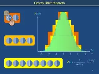
Meditation about the CLT Can a large group of insane individuals behave as reasonably as a randomly chosen groupe of IBM or NASA engineers ?
As a matter of fact. CLT indicates that such an assumption is not completely unreasonable. According to CLT, “the sums of independent random variables tend to look normal no matter what crazy distribution the individual variables have” (G&S,p.362).
Question for practice (G&S,9.3.7) Extra-credit • Choose independently 25 numbers from the interval [0,1] with the probability density f(x) given below and compute their sum s25. Repeat this experiment 100 times and make a bar graph of the result. How well does the normal density fit your bar graph in each case? • f(x)=1 • f(x) = 3 x2 • f(x) = 2 - 4|x-1/2|
Confidence Interval In statistics we always deal with the limited samples of population. Usually, the goal is to draw inferences about a population from a sample. This approach is called “Inferential statistics”. Suppose that we are interested in the mean number of words that can be remembered by a high school student. First, we have to select a random sample from the population. Suppose that the group of 15 students is chosen. We can use the sample mean as an unbiased estimate of , the population mean value. However, given the small size of the sample, it will certainly not be a perfect estimate. By chance it is bound to be at least either a little bit too high or a little bit too low.
For the estimate of μ to be of value, one must have some idea of how precise it is. That is, how close to μ is the estimate likely to be? The CLT helps answering this question. It tells us that the sample mean is a random variable normally distributed near the population mean. This can help us to derive a probabilistic estimate of μ based on the sample mean. An excellent way to specify the precision is to construct a confidence interval. 4.1 Confidence interval, is known Let’s assume for simplicity that we have to estimate μ while is known (this case is not very realistic but can give us an idea).
It can be shown (check it with Mathematica) that for the standard normal distribution * Noticing now that the standardized variable is we have *More precisely, the 95% range is (-1.96, 1.96), but using (-2,2) is good enough for all practical purposes
In other words, with the probability ~0.95, belongs to the interval We say that this is a 95% confidence interval for
Example 1. Suppose that we have a random sample of size 100 from a population with standard deviation 3 and we observe a sample mean . What can we tell about μ? In this case As a result,
Example 2. How large a sample must be selected from a normal distribution with standard deviation 12 in order to estimateto within 2 units
In the previous example it was assumed that the Variance is known. It is much more common that neither mean nor the variance is known when the sampling is done. As a rough estimate, one can use the sample variance: This will lead to a normalized variable Which is a function of two random variables.
It was shown by W.S. Gosset that the density function for Tn is not normal but rather a t-density with n degrees of freedom. For large n t-density approaches the normal distribution. In general, t-density closely related the Chi-squared distribution This is called the Chi-squared distribution with n degrees of freedom.
This distribution describes the sum of squares of n independent random variables. It is very important for comparing experimental data with a theoretical discrete distribution to see whether the data support the theoretical model. Please read Chapter 7.2 of G&S for details. Here we consider only simple examples of hypothesis testing.
Hypothesis testing We consider now two types of hypothesis testing: Testing the mean and testing the difference between two means
Example 1. Suppose we run a casino and we wonder if our roulette wheel is biased. To rephrase our question in statistical terms, let p be the probability red comes up and introduce two hypothesis H0: p = 18/38 null hypothesis H1: p 18/38 alternative hypothesis To test to see if the null hypothesis is true, we spin the roulette n times and let Xi=1 if red comes up on the i-th trial and 0 otherwise, so that (the observed mean value) is the fraction of times red came up in the first n trials.
How to decide if H0 is correct? It is reasonable to suggest that large deviations of from the “fair” value 18/38 would indicate that H0 failed. But how to decide which deviations should be considered “large”? The concept of the “confidence interval” can help answering this question. As we know, with probability ~95% should belong to the confidence interval Reminder: n is the sampling size or the number of the iid (independent and identically distributed) variables added together, and are their individualmean and standard deviation values.
Rejecting H0 when it is true is called a type I error. Accepting H0 when the alternative hypothesis is true is called a type II error In this test we have set the type I error to be 5% Thus, we can say that if falls outside the chosen interval, then the H0 can be rejected with possible error less then 5%. Let us find now the individual standard deviation. The variable Xitakes only two values: 0 and 1. Probability(1)=18/38, Probability(0)= 20/38. Using this, we can find <Xi2>= 1*18/38+0*20/38=18/38. (I use <…> notation for the mean.)
Thus, 2 σ ~ 1 and the test can now be formulated as: or in terms of the total number of reds Sn = S1 +S2+ … Sn,
Suppose that we spin the wheel 3800 times and get red 1869 times. Is the wheel biased? The expected number of reds is (18/38)n=1800. Is the deviation from this value | Sn – 1800| = 69 indicates that the wheel is biased? Given the large numbers of trials, this deviation might not seem large. However, it must be compared with n1/2 = (3800)1/2 ~ 61.6 Given that 69 > 61.6 we have to reject H0 with a notion that if H0 were correct then we would see and observation this far from the mean less than 5% of the time. Obviously, it does not prove the wheel is biased but shows that it is very likely to be true.
Example 2. Do married college students with children do less well because they have less time to study or do they do better because they are more serious? The average GPA for all students was 2.48. To answer the question, we formulate two hypothesis: H0: = 2.48 null hypothesis H1: 2.48 alternative hypothesis
The records of 25 married college students with children indicate that their GPA average was 2.36 with the standard deviation of 0.5. Using the last example, we see that to derive a conclusion with type I error of 5% we should reject H0 if We can see that the observed deviation |Xi -2.48|=0.12 < 0.2. It means that we can not reject the 0-hypothesis. In other words, we can not be 95% certain that married students with children do either worth or better that the students without children.
Testing the difference of two means Suppose that we want to compare the test results for two independent random samples of size n1 and n2 taken from two different populations. A typical example would be testing a drug, one sample taken from the population taking the drug and another – from the reference group. Suppose now that the population means are unknown. For example, we do not know what % of population would be infected by a certain disease if the drug is not taken. Notice that in the previous case we were able to calculate the mean for the 0-hypothesis. Now we can not.
H0 : - null hypothesis H1 = - alternative hypothesis From the CLT: - If H0 correct, then
Based on the last result, if we want a test with a type 1 error of 5% then we should reject H0 if Example: study of passive smoking reported in NEJM. The size of lung airways was taken for 200 female nonsmokers who were in a smoky environment and for 200 who were not. For the 1-st group the average was 2.72 and sigma= 0.71, while for the second group the corresponding values were 3.17 and 0.74.
Based on these data we find while This means that the conclusions are convincing (should be taken seriously)