Download

1 / 15
160 likes | 403 Vues
Gridded Population of the World. Version 2: 1995 UN adjusted population density Gridded Population Workshop May 2-3, 2000. GPW Version 2 Characteristics:. Based on national and sub-national spatial and population data, best available or ‘affordable’

E N D
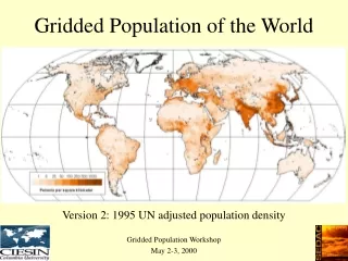
Gridded Population of the World Version 2: 1995 UN adjusted population density Gridded Population Workshop May 2-3, 2000
GPW Version 2 Characteristics: • Based on national and sub-national spatial and population data, best available or ‘affordable’ • Data set of quadrilateral grids (2.5’, or 20 km2 at equator) that contain estimates of: • population (1990 and 1995, raw and adjusted) • land area (administrative unit area net of lakes) • Six continents covered (Antarctica was not gridded)
Best available ‘matched’ data used (population and boundaries must match) Commercial, government and other institutional sources over 100 sources roughly 40 data suppliers Source Data Characteristics
Population Data Adjustments Definitions r Annual rate of growth P1..2 Census estimate t number of years between census enumerations Px Year of Estimate (90 or 95) Pun UN Estimate Padj Adjusted estimate • Annual rate of change calculated: • Population estimates adjusted to 1990 and 1995: Px = P2 ert
Population Data Adjustments • Adjustment factor for matching national estimates to UN estimates calculated: a = (Pun - Px) / Pun • Adjustment factor applied at the national level : Padj = Px * a Definitions a Adjustment factor Px Year of Estimate (90 or 95) Pun UN Estimate Padj Adjusted estimate
Source Boundary Data Administrative unit centroids shown for the approximately 127,000 units collected for GPW v2
Boundary Data Adjustments • International boundaries and coastlines matched to the Digital Chart of the World (DCW): • completed without data loss • some countries left unmatched (e.g., SABE data) • Lakes and ice from DCW added to boundary data
Gridding Algorithm • Proportional allocation used to spread the population over grid cells • Virtually all data work completed on vector data; gridding is the last step. • National grids created, global grids assembled by adding national grids together • country grids are created with collars so that they start and end on even degrees; therefore the assembly of the grids without interpolation is possible
Gridding Algorithm: Proportional Allocation • Adjusted boundary data is unioned with a blank fishnet coverage of grid cells • Resulting small polygons have areas and densities calculated
Gridding Algorithm • Population densities (input and adjusted) are multiplied by the polygon areas to allocate population • Result is a detailed coverage with population estimates for each polygon • Population and area information are then gridded
Issues in Adjusting Population Data • Variable quality source census data • Timeliness of input data varies • Additional demographic data are not available to improve estimates • available in sample surveys • limited coverage (although tend to be strong where census data are weak) • nationally or sub-nationally representative, but usually not representative beyond administrative level 2
Issues in Adjusting Boundary Data/Gridding • Small rounding error introduced • Variable quality and detail of input data degrades final product • Process intensive (cpu and storage)
Possible Improvements • Better source data (boundary and census) • Additional spatial inputs, e.g.,: • parks (constraint) • roads, populated places (‘attractors’ in a heuristic model) • Additional population inputs, e.g.,: • Survey data • Grid other variables • demographic, socioeconomic, etc • Custom grids