Chapter 11: Population Growth
460 likes | 786 Vues
Chapter 11: Population Growth. Geometric Rate of Increase. Geometric Rate of Increase ( λ ): λ =N t+1 / N t N t+1 = Size of population at future time. N t = Size of population at some earlier time. Non-overlapping generations Determines the rate of population growth. Geometric Growth.

Chapter 11: Population Growth
E N D
Presentation Transcript
Geometric Rate of Increase • Geometric Rate of Increase (λ): • λ=N t+1 / Nt • N t+1 = Size of population at future time. • Nt = Size of population at some earlier time. • Non-overlapping generations • Determines the rate of population growth
Geometric Growth • When generations do not overlap, growth can be modeled geometrically. Nt = Noλt • Nt = Number of individuals at time t. • No = Initial number of individuals. • λ = Geometric rate of increase. • t = Number of time intervals or generations.
Geometric Rate of Increase Phlox drummondii
Predator populations are also known to increase in geometric fashion when released into favorable sites.
Rate of Increase • Per Capita Rate of Increase (r): • r = ln Ro / T • ln = Base natural logarithms • Actual, or realized, rate of increase determined from actual life table data • Growth = rN • Intrinsic Rate of Increase • rmax • Maximum per capita rate of increase • Occurs under ideal environmental conditions with constant birth rates, death rates, and age structures
Unlimited Population Growth Much depends on the value of R0: • In the simplest models, R0 remains constant. • When R0 < 1, the population eventually declines to extinction. • When R0 > 1, the population increases. • When R0 = 1, the population is at equilibrium, where no changes in population density occur.
Unlimited Population Growth Describes population growth for continuous breeders • For small organisms, such as bacteria, internal parasites, or humans, reproduction can be continuous. • To understand population growth under these conditions, a slightly different type of model is required.
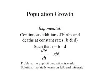
Exponential Growth • Continuous population growth in an unlimited environment can be modeled exponentially. dN / dt = rmax N • Appropriate for populations with overlapping generations. • As population size (N) increases, rate of population increase (dN/dt) gets larger.
Exponential Growth • For an exponentially growing population, size at any time can be calculated as: Nt = Noermaxt • Nt = Number individuals at time t. • N0 = Initial number of individuals. • e = Base of natural logarithms. • rmax = Per capita rate of increase. • t = Number of time intervals. • Terminated when population exceeds the number that the habitat can support
Exponential Growth R0 and r are similar • R0 reflects a generational growth rate • r, denotes an instantaneous rate. Dividing the natural log of R0 by the generation time gives us r: Thus, r ≈ ln R0 T
Exponential Growth How do populations of continuous breeders grow? • Much depends on the value of r. • When r < 0, the population decreases. • When r = 0 the population remains constant. • When r > 0 the population increases When r = 0, the population is referred to as being at equilibrium. Where no changes in population size will occur and there is zero population growth.
Exponential Growth Rate Can this continue indefinitely?
Exponential Population Growth This is a common trend when populations successfully colonize new territory.
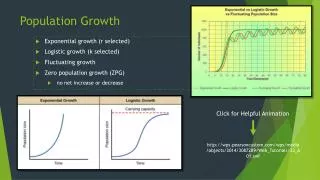
Unlimited Population Growth Leads to “J”-shaped population growth curves. • The greater the population growth rate, the faster a population grows. • When a population breeds seasonally (often once a year) we say the population grows geometrically. • Some species reproduce almost continuously and generations overlap. We say these populations grow exponentially. • Both geometric and exponential growth produce “J”-shaped population growth curves.
Carrying Capacity • Carrying Capacity (K)- The maximum rate of animal stocking possible without inducing damage to the vegetation or related resources • may vary from year to year because of fluctuating forage production. • K is a determined by a specific habitat for each species • What environmental factors determine K? • Range condition / vegetation (most common) • Disease? • Social tolerance and distribution? • Et cetera, et alias
Logistic Population Growth • As resources are depleted, population growth rate slows and eventually stops = logistic population growth. • Sigmoid (S-shaped) population growth curve. • Carrying capacity (K) is the number of individuals of a population the environment can support. • Finite amount of resources can only support a finite number of individuals.
Logistic Population Growth • Continuous breeders have a per capita growth rate, r. • Logistic growth, which takes into account the amount of available resources, is given by: Per capita rate of population growth Population size dN = rN (K – N) dtK Rate of population change Carrying capacity
Logistic Population Growth dN/dt = rmaxN(K-N/K) • rmax = Maximum per capita rate of increase under ideal conditions. • When N approaches K, the right side of the equation nears zero. • As population size increases, logistic growth rate becomes a small fraction of possible growth rate. • Highest growth rate when N=K/2. • N/K = Environmental resistance.
Inflection Point Logistic Curve
Logistic Population Growth • If K = 1,000 and population sizes are low (N=100), even though (K-N)/K is close to 1, population sizes are so small that growth is small. If K = 1,000, N = 100 and r = 0.1 then dN= (0.1) (100) x (1,000 100) dt 1,000 = 9
Logistic Population Growth • At medium values of N, (K-N)/K is less close to a value of 1 but population growth is larger because there are a larger number of reproducing females. If K = 1,000, N = 500 and r = 0.1 then dN= (0.1) (500) x (1,000 500) dt 1,000 = 25
Logistic Population Growth • At larger values of N, (K-N)/K becomes small, resources are close to being used up, and population growth is again small. If K = 1,000, N = 900 and r = 0.1 then dN= (0.1) (900) x (1,000 900) dt 1,000 = 9
Logistic Population Growth Balanus balanoides Paramecium caudatum
Population Growth • In reality, populations do not grow in a perfectly logistic fashion – they tend to grow in a more non-symmetrical fashion
Variation in abundance of different species of small mammal populations over many years of data collection. As seen here, the data shows great variability and a lack of fit to the idealized logistic growth curve. Data reflect relative abundance in a set number of traps at different sampling points. What about time lags?
Doubling Time • Once r is known, then the population doubling time can be calculated. • The equation is often approximated as: d = 0.7/r • This relationship is called “the rate of 70.” • Take 70 and divide it by the growth rate • The growth rate is cast as the percentage increase in a year.
Doubling Time • Example of “the rate of 70” • In 2006, the world’s population grew by 1.23%. If that rate was to continue unchanged, the world’s population would double in 57 years, because • 70/1.23 = 57 • You can make a similar calculation about accrual of money in a savings account. If your bank pays you 5% interest, your money will double in • 70/5=14 years
Limits to Population Growth • Environment limits population growth by altering birth and death rates. • Density-dependent factors • Disease • Resource competition • et cetera • Density-independent factors • Natural disasters • Weather • et cetera
Density-Dependent Factors • Birth rates may decrease as populations increase because resources become more limited and density-dependent competition for those resources increases. • Density-dependent mortality may also occur as population densities increase and competition for resources increases, reducing offspring production or survival.
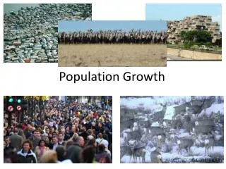
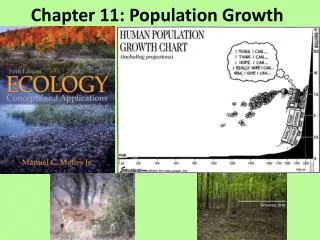
Human Population Growth • In 2006, the world’s population was increasing at the rate of 146 people every minute. • Projections pointed to the human population stabilizing at around 10 billion near the year 2150. • Between 1750 and 1998 the world’s human population surged from 800 million to 6 billion. • In 2009 the number of humans was estimated at 6.7 billion.
Statistical Significance • Statistical Significance (P-Values) • Results are statistically significant if they are unlikely to have occurred by chance • “A measure of how unlikely it is that a result has occurred by chance” • P<0.05 is traditional • Less than 1 chance in 20 that the observed results happened by chance • Anything less is said to be statistically significant.
chi-square (χ2)“goodness of fit” test • Tests the relationship between observed and hypothesized frequency • Are organisms being selective or using environmental factors in the proportion of availability? • Do laying turtles prefer sandy soil over clay soils? • Does a bird species prefer sweetgum over other species of trees? • Do honeybees choose higher cavities than lower cavities? • Do red-colored males get more mates than orange-colored males? • Does a bird species really prefer seeds of a certain size or type? • ……..or are observations due just to differential availability of resources?
chi-square (χ2)“goodness of fit” test You go out and determine the date of flowering in 75 Blessed Milk Thistles (Silybum marianum). You know that they flower from June through August, and you want to know if they flower equally or not. χ2 = ∑[(0-E)2/E]
chi-square (χ2)“goodness of fit” test χ2 = ∑[(0-E)2/E] = χ2 = [(7-25)2/25]+ [(53-25)2/25]+ [(15-25)2/25] = χ2 = [(-18)2/25]+ [(28)2/25]+ [(-10)2/25] = χ2 = [324/25]+ [784/25]+ [100/25] = χ2 =13+31.36+4 = χ2 =48.36 • Use a P-Value of 0.05 to determine significance. • Determine the degrees of freedom (i.e., the number of phenotypes minus one, or n-1 • 3-1 = 2 degrees of freedom. • See a table of Critical Values of Chi-Square (page 540)
Since our computed χ2 =48.36 is greater than the predicted value of 5.99, we reject the hypothesis that the thistle plants flower in equal frequencies during the months of June through August.