Download
1 / 44
440 likes | 653 Vues
Analysis of the terrestrial carbon cycle through data assimilation and remote sensing. Mathew Williams, University of Edinburgh Collaborators L Spadavecchia, M Van Wijk. B Law, J Irvine, P Schwarz, M Kurpius, T Quaife, P Lewis M Disney G Shaver, L Street.

E N D
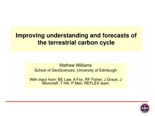
Analysis of the terrestrial carbon cycle through data assimilation and remote sensing Mathew Williams, University of Edinburgh Collaborators L Spadavecchia, M Van Wijk. B Law, J Irvine, P Schwarz, M Kurpius, T Quaife, P Lewis M Disney G Shaver, L Street
Sampling at 3397 meters, well mixed free troposphere Source: CD Keeling, NOAA/ESRL
Harvard Forest Data since 1989
Hourly data ~5 m above canopy Source: Wofsy et al, Harvard Forest LTER
Talk outline What are the uncertainties in temporal and spatial extrapolation of C cycle estimates? • Using multiple time series data to constrain C cycle analyses • Use multiscale spatial studies to determine up-scaling uncertainties
FUSION ANALYSIS ANALYSIS + Complete + Clear confidence limits + Capable of forecasts Improving estimates of C dynamics MODELS MODELS + Capable of interpolation & forecasts - Subjective & inaccurate? OBSERVATIONS +Clear confidence limits - Incomplete, patchy - Net fluxes OBSERVATIONS
A prediction-correction system Time update “predict” Measurement update “correct” Initial conditions
The Kalman Filter Initial state Drivers Forecast Observations Predictions At Ft+1 Dt+1 F´t+1 MODEL OPERATOR P Assimilation Ensemble Kalman Filter At+1 Analysis
C cycling in Ponderosa Pine, OR Flux tower (2000-2) Sap flow Soil/stem/leaf respiration LAI, stem, root biomass Litter fall measurements
Sap-flow A/Ci Chambers Chambers EC Time (days since 1 Jan 2000) Williams et al GCB (2005)
Rtotal & Net Ecosystem Exchange of CO2 Af Lf Cfoliage Rh Ra Ar Lr GPP Croot Clitter D 5 model pools 10 model fluxes 11 parameters 10 data time series Aw Lw Cwood CSOM/CWD C = carbon pools A = allocation L = litter fall R = respiration (auto- & heterotrophic) Temperature controlled
= observation — = mean analysis | = SD of the analysis Time (days since 1 Jan 2000) (Williams et al 2005)
= observation — = mean analysis | = SD of the analysis Time (days since 1 Jan 2000) (Williams et al 2005)
Data brings confidence =observation — = mean analysis | = SD of the analysis (Williams et al 2005)
At Ft+1 Reflectancet+1 MODISt+1 DALEC Radiative transfer DA At+1 Assimilating EO reflectance data
GPP results No assimilation Assimilating MODIS (bands 1 and 2) Quaife et al, RSE (in press)
Summary: time • Multiple time series data generate powerful constraints on analyses • For improved predictions, better constraints on long time constant processes are required • Error characterisation is vital • EO data can be assimilated with appropriate observation operators
Height of sensor and field of view 3.0 m 2.0 m 1.5 m 1.0 m 0.5 m 0.2 m 4.5 m 3.0 m 2.35 m 1.5 m 0.75 m 0.1 m
A multi-scale experimental design macroscale microscale Distance (m) Distance (m) (Williams et al. in press)
Microscale study: Scale invariance Linear averaged Skye NDVIs (collected at 0.2 x 02 m resolution with diffuser off) versus measured NDVIs at coarser spatial scales with diffuser on
Microscale study: Scale invariance Relationships between estimated LAI (using both Skye NDVI and LI-COR LAI-2000 observations at 0.2 m resolution, linearly averaged for upscaling) versus Skye NDVI at different spatial scales.
Frequency histograms for LAI estimates in the microscale site at a range of resolutions. (Williams et al. in press)
Macroscale study: Frequency histograms Inferred from ground NDVI Measured in a ground survey, 2004 Satellite overpass, ETM+, August 2001
Macroscale study: Semivariograms Inferred from ground NDVI Measured in a ground survey, 2004 Satellite overpass, ETM+, August 2001
Landsat IDW Kriging Kriging Error (Williams et al. in press)
Summary: space • Scale invariance in LAI-NDVI relationships at scales > vegetation patches • However spatial variability is high so Kriging has limited usefulness • Over scales >50 m interpolation error was of similar magnitude to the uncertainty in the Landsat NDVI calibration to LAI • Characterisation of spatial LAI errors provides key data for spatial data assimilation
Key challenges and opportunities • Coping with variable data richness • Identifying and removing model bias • Estimating representation and data errors • Making use of remote sensing (optical and XCO2) • Links to atmospheric CO2 using CTMs. • Designing experimental network • Boundaries in natural systems
Funding support: NERC NASA DOE Thank you
REFLEX: GOALS • To identify and compare the strengths and weaknesses of various MDF techniques • To quantify errors and biases introduced when extrapolating fluxes made at flux tower sites using EO data • Closing date for contributions: 31 October www.carbonfusion.org
Regional Flux Estimation Experiment, stage 1 Flux data MODIS LAI Training Runs - FluxNet data - synthetic data Assimilation MDF DALEC model Deciduous forest sites Coniferous forest sites Output Full analysis Model parameters Forecasts www.carbonfusion.org
Figure by Andrew Fox observations (with noise) truth predictions uncertainty Synthetic evergreen forest 2 years obs., 1 year prediction
REFLEX, stage 2 Flux data MODIS LAI Testing predictions With only limited EO data MDF Flux data DALEC model testing MDF Model parameters Analysis Assimilation MODIS LAI
FluxNet – Integrating worldwide CO2 flux measurements How to upscale from site locations to regions and the globe?