Download
1 / 25
250 likes | 359 Vues
Explore the challenges of flux tower data assimilation for accurate carbon cycle modeling. Utilize innovative strategies to incorporate both fast and slow processes for real-time source/sink mapping. Implement advanced modeling and analysis tools to optimize CO2 simulations and improve estimation accuracy.

E N D
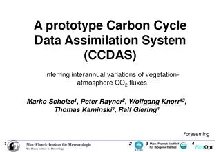
Space-Time Variability in Carbon Cycle Data Assimilation Scott Denning, Peter Rayner, Dusanka Zupanski, Marek Uliasz, Nick Parazoo, Ravi Lokupitiya, Andrew Schuh, Ian Baker, and Ken Davis Acknowledgements: Support by US NOAA, NASA, DoE
Regional Fluxes are Hard! • Eddy covariance flux footprint is only a few hundred meters upwind • Heterogeneity of fluxes too fine-grained to be captured, even by many flux towers • Temporal variations ~ hours to days • Spatial variations in annual mean ~ 1 km • Some have tried to “paint by numbers,” • measure flux in a few places and then apply everywhere else using remote sensing • Annual source/sink isn’t a result of vegetation type or LAI, but rather a complex mix of management history, soils, nutrients, topography not easily seen by RS
A Different Strategy • Divide carbon balance into “fast” processes that we know how to model, and “slow” processes that we don’t • Use coupled model to simulate fluxes and resulting atmospheric CO2 • Measure real CO2 variations • Figure out where the air has been • Use mismatch between simulated and observed CO2 to “correct” persistent model biases • GOAL: Time-varying maps of sources/sinks consistent with observed vegetation, fluxes, and CO2 as well as process knowledge
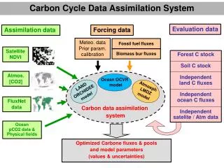
Modeling & Analysis Tools(alphabet soup) • Ecosystem model (Simple Biosphere, SiB) • Weather and atmospheric transport (Regional Atmospheric Modeling System, RAMS) • Large-scale continental inflow (Parameterized Chemical Transport Model, PCTM) • Airmass trajectories(Lagrangian Particle Dispersion Model, LPDM) • Optimization procedure to estimate persistent model biases upstream (Maximum Likelihood Ensemble Filter, MLEF)
SiB SiB unknown! unknown! Flux-convolved influence functions derived from SiB-RAMS Treatment of Variations for Inversion • Fine-scale variations (hourly, pixel-scale) from weather forcing, NDVI as processed by forward model logic (SiB-RAMS) • Multiplicative biases (caused by “slow” BGC that’s not in the model) derived by from observed hourly [CO2]
Continental NEE and [CO2] • Variance in [CO2] is strongly dominated by diurnal and seasonal cycles, but target is source/sink processes on interannual to decadal time scales • Diurnal variations are controlled locally by nocturnal stability (ecosystem resp is secondary!) • Seasonal variations are controlled hemispherically by phenology • Synoptic variations controlled regionally, over scales of 100 - 1000 km. Let’s target these.
Seasonal and Synoptic Variations Daily min [CO2], 2004 • Strong coherent seasonal cycle across stations • SGP shows earlier drawdown (winter wheat), then relaxes to hemispheric signal • Synoptic variance of 10-20 ppm, strongest in summer • Events can be traced across multiple sites • “Ring of Towers” in Wisconsin
Lateral Boundary Forcing • Flask sampling shows N-S gradients of 5-10 ppm in [CO2] over Atlantic and Pacific • Synoptic waves (weather) drive quasi-periodic reversals in meridional (v) wind with ~5 day frequency • Expect synoptic variations of ~ 5 ppm over North America, unrelated to NEE! • Regional inversions must specify correct time-varying lateral boundary conditions • Sensitivity exp: turn off all NEE in Western Hemisphere, analyze CO2(t)
SiB-RAMS Simulated Net Ecosystem Exchange (NEE) Average NEE
Ring of Towers: May-Aug 2004 • 1-minute [CO2] from six 75-m telecom towers, ~200 km radius • Simulate in SiB-RAMS • Adjust (x,y) to optimize mid-day CO2 variations
Back-trajectory “Influence Functions” • Release imaginary “particles” every hour from each tower “receptor” • Trace them backward in time, upstream, using flow fields saved from RAMS • Count up where particles have been that reached receptor at each obs time • Shows quantitatively how much each upstream grid cell contributed to observed CO2 • Partial derivative of CO2 at each tower and time with respect to fluxes at each grid cell and time
no info over Great Lakes Wow!
Next Step: Predict • If we had a deterministic equation that predict the next from the current we could improve our estimates over time • Fold into model state, not parameters • Spatial covariance would be based on “model physics” rather than an assumed exponential decorrelation length • Assimilation will progressively “learn” about both fluxes and covariance structure
CSU RAMS (T, q) Winds Clouds CO2 Transport and Mixing Ratio PBL Precipitation Radiation Surface layer H LE NEE SiB3 Canopy air space Leaf T Sfc T CO2 Photosynthesis CO2 Snow (0-5 layers) Soil T & moisture (10 layers) autotrophic resp allocation Biogeochemistry Leaves Wood Roots Litter pools heterotrophic resp Microbial pools Slow soil C passive soil C Coupled Modeling and Assimilation System • Adding C allocation and biogeochemistry to SiB-RAMS • Parameterize using eddy covariance and satellite data • Optimize model state variables (C stocks), not parameters or unpredictable biases • Propagate flux covariance using BGC instead of a persistence forecast
Summary/Recommendations • Space/time variations of NEE are complex and fine-grained, resulting from hard-to-model processes • Variations in [CO2] dominated by “trivial” diurnal & seasonal cycles that contain little information about time-mean regional NEE • Target synoptic variations to focus on regional scales • Model parameters control higher-frequency variability … optimize against eddy flux & RS • Time-mean NEE(x,y) depends on BGC model state (C stocks) rather than parameters … optimize these based on time-integrated model-data mismatch • 70 days of 2-hourly data sufficient to estimate stationary model bias on 20-km grid over 360,000 km2