Download
1 / 26
260 likes | 396 Vues
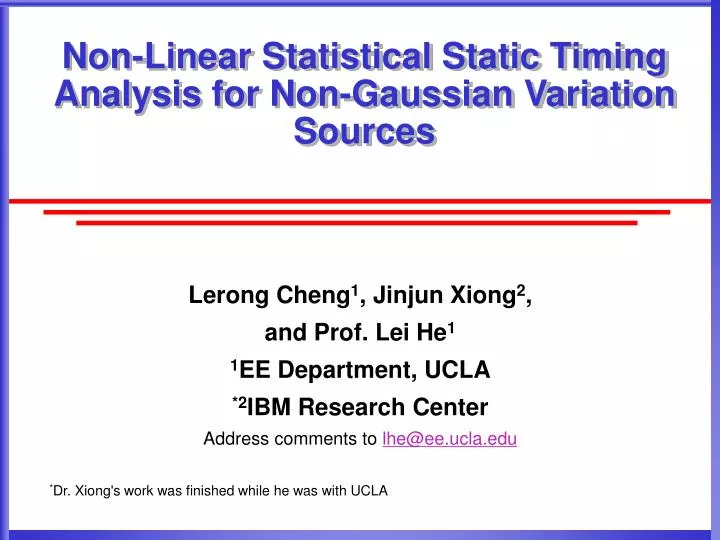
Non-Linear Statistical Static Timing Analysis for Non-Gaussian Variation Sources. Lerong Cheng 1 , Jinjun Xiong 2 , and Prof. Lei He 1 1 EE Department, UCLA *2 IBM Research Center Address comments to lhe@ee.ucla.edu * Dr. Xiong's work was finished while he was with UCLA. Outline.

E N D
Non-Linear Statistical Static Timing Analysis for Non-Gaussian Variation Sources Lerong Cheng1, Jinjun Xiong2, and Prof. Lei He1 1EE Department, UCLA *2IBM Research Center Address comments to lhe@ee.ucla.edu *Dr. Xiong's work was finished while he was with UCLA
Outline • Background and motivation • Delay modeling • Atomic operations for SSTA • Experimental results • Conclusions and future work
Motivation • Gaussian variation sources • Linear delay model, tightness probability [C.V DAC’04] • Quadratic delay model, tightness probability [L.Z DAC’05] • Quadratic delay model, moment matching [Y.Z DAC’05] • Non-Gaussian variation sources • Non-linear delay model, tightness probability [C.V DAC’05] • Linear delay model, ICA and moment matching [J.S DAC’06] • Need fast and accurate SSTA for Non-linear Delay model with Non-Gaussian variation sources not all variation is Gaussian in reality computationally inefficient
Outline • Background and motivation • Delay modeling • Atomic operations for SSTA • Experimental results • Conclusions and future work
Delay Modeling • Delay with variation • Linear delay model • Quadratic delay model • Xis are independent random variables with arbitrary distribution • Gaussian or non-Gaussian
Outline • Background and motivation • Delay modeling • Atomic operations for SSTA • Max operation • Add operation • Complexity analysis • Experimental results • Conclusions and future work
Max Operation • Problem formulation: • Given • Compute:
Reconstruct Using Moment Matching • To represent D=max(D1,D2) back to the quadratic form • We can show the following equations hold • mi,k is the kth moment of Xi, which is known from the process characterization • From the joint moments between D and Xis the coefficients ais and bis can be computed by solving the above linear equations • Use random term and constant term to match the first three moments of max(D1, D2)
Basic Idea • Compute the joint PDF of D1 and D2 • Compute the moments of max(D1,D2) • Compute the Joint moments of Xi and max(D1,D2) • Reconstruct the quadratic form of max(D1,D2) • Keep the exact correlation between max(D1,D2) and Xi • Keep the exact first-three moments of max(D1,D2)
JPDF by Fourier Series • Assume that D1 and D2 are within the ±3σ range • The joint PDF of D1 and D2, f(v1, v2)≈0, when v1 and v2 is not in the ±3σ range • Approximate the Joint PDF of D1 and D2 by the first Kth order Fourier Series within the ±3σ range: where , αij are Fourier coefficients
Fourier Coefficients • The Fourier coefficients can be computed as: • Considering outside the range of where • can be written in the form of . • can be pre-computed and store in a 2-dimensional look up table indexed by c1 and c2
JPDF Comparison • Assume that all the variation sources have uniform distributions within [-0.5, 0.5] • Our method can be applies to arbitrary variation distributions • Maximum order of Fourier Series K=4
Moments of D=max(D1, D2) • The tth order raw moment of D=max(D1,D2) is • Replacing the joint PDF with its Fourier Series: where • L can be computed using close form formulas • The central moments of D can be computed from the raw moments
Joint Moments • Approximate the Joint PDF of Xi, D1, and D2 with Fourier Series: • The Fourier coefficients can be computed in the similar way as • The joint moments between D and Xis are computed as: • Replacing the f with the Fourier Series where
PDF Comparison for One Step Max • Assume that all the variation sources have uniform distributions within [-0.5, 0.5]
Outline • Background and motivation • Delay modeling • Atomic operations for SSTA • Max operation • Add operation • Complexity analysis • Experimental results • Conclusions and future work
Add Operation • Problem formulation • Given D1 and D2, compute D=D1+D2 • Just add the correspondent parameters to get the parameters of D • The random terms are computed to match the second and third order moments of D
Complexity Analysis • Max operation • O(nK3) Where n is the number of variation sources and K is the max order of Fourier Series • Add operation • O(n) • Whole SSTA process • The number of max and add operations are linear related to the circuit size
Outline • Background and motivation • Delay modeling • Atomic operations for SSTA • Experimental results • Conclusions and future work
Experimental Setting • Variation sources: • Gaussian only • Non-Gaussian • Uniform • Triangle • Comparison cases • Linear SSTA with Gaussian variation sources only • Our implementation of [C.V DAC04] • Monte Carlo with 100000 samples • Benchmark • ISCAS89 with randomly generated variation sensitivity
PDF Comparison • PDF comparison for s5738 • Assume all variation sources are Gaussian
Mean and Variance Comparison for non-Gaussian Variation Sources
Outline • Background and motivation • Delay modeling • Atomic operations for SSTA • Experimental results • Conclusions and future work
Conclusion and Future Work • We propose a novel SSTA technique is presented to handle both non-linear delay dependency and non-Gaussian variation sources • The SSTA process are based on look up tables and close form formulas • Our approach predict all timing characteristics of circuit delay with less than 2% error • In the future, we will move on to consider the cross terms of the quadratic delay model