Efficient Timing Analysis Methods for Design Optimization
Understand static and dynamic timing analysis, gate delay models, critical paths, wire delays, slack, false paths, and how to optimize timing in circuit design for efficient performance. Learn the algorithms and techniques for accurate timing predictions.

Efficient Timing Analysis Methods for Design Optimization
E N D
Presentation Transcript
Timing analysis • Need to know the clock frequency in the design process • Dynamic Timing Analysis: • Simulation: • Needs input vectors (not known during design process) • Can miss an obscure performance-limiting path • Very slow • Impractical in the loops of design phases
Timing analysis • Static Timing Analysis (STA): • Fast • Reasonably accurate measurement of timing • Simplified delay models • Calculates an upper bound on frequency • Conservative analysis • Safe: guarantees that the design will function at least as fast as predicted • Delay characterization for cell libraries is clearly defined • Forms an effective interface between the foundry and the design team
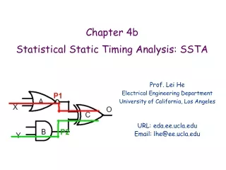
STA • Combinational circuits: Graph model: DAG • Vertices: • I/O pins of gates • s and t • Edges: • Connect each input of a gate to its output • Show maximum delay paths from the input pin to the output pin • Connects the output of each gate to the inputs of its fanout gates • Show interconnect delays • In case of combinational loop: • Many STA tools break the loop and analyze
STA Timing Graph • Simplified graph 2 3 6 4 2 s 2 5 3
Sequential Circuits • Represented as: • a set of combinational blocks that lie between latches. • A timing graph may be constructed for each of these blocks • Inputs of graph: PIs + FF outputs • Outputs of graph: POs + FF inputs
Sequential Circuits • Algorithm for finding combinational blocks: • Construct a graph in which each vertex corresponds to a combinational element, • An undirected edge is drawn between a combinational element and the combinational elements that it fans out to • Sequential elements are left unrepresented • The connected components of this graph correspond to the combinational blocks
Gate Delay Models • Methods for calculating gate delay: • Look-up table method: • Each entry: delay under different capacitive loads and input transition times. • Good accuracy • But memory-intensive • Linear model: • Traditional: (k1 CL + k2): • k1: characterized slope • k2: intrinsic delay • Neglects the effect of the input transition time • k-factor equations: • Compact the table look-up by fitting function to • (k1 + k2CL)τin + k3CL3 + k4CL + k5
STA Algorithm • Traverse in topological order • Apply: 10
STA Algorithm 0 2 2 13 0 3 6 0 6 17 0 10 4 2 0 2 2 0 15 5 0 3 3 0 Wire delays ignored or added to the gate delays
STA: Critical Path • Critical path: • Trace back from the PO with largest arrival time • This is the output of last block on critical path • Identify the latest arriving input of the block • Identify the block that causes this transition • Repeat
Critical Path: Example 0 2 2 13 0 3 6 0 6 17 0 10 4 2 0 2 2 0 15 5 0 3 3 0
Required Arrival Times • If Timing constraints are specified: • For each node, must check if met or not • Useful to know which parts should be sped up • If ATnode > RTnode, the path that the node lies on must be sped up
Required Arrival Times 13 15 • Consider delays as –ve • Apply the same procedure from output to inputs • Arrow directions reversed 2 18 13 3 9 3 6 20 3 Min(15,13) = 13 4 2 7 9 2 7 18 5 10 13 3 10
Slack • Slack of a node: • RTnode – ATnode • +ve slack s: • Arrival time of that node can be increased by s w/o affecting the overall delay of circuit • Potential to optimize power/area/…. • In FPGAs, >75% of nodes have ~ 50% slack
Incremental STA • In physical design loops: • A small change in module locations/connection paths • In design flow: • A small change in circuit • No need for full STA • Incremental STA: • Event-driven procedure: • An event occurs when timing info at the input to the gate is changed • Only a small fraction of gates have their arrival times changed
d = 10 d = 10 d = 20 d = 20 False path False Paths • Many paths never occur • Considering them pessimistic may waste resources • Assumption: • INV delay = 0 • Critical path: 40 • May try too hard to optimize it
False Paths • Solutions: • Automatic solutions: too complex to be practical • E.g. if inverter delay > 0 • In practice: • Designers knows functionalities best Designer specifies
References • [Sapatnekar06] Sapatnekar, “Static Timing Analysis,” EDA for IC Implementation, Circuit Design, and Process Technology, 2006.