Static Timing Analysis for Combinational Threshold Logic Networks
740 likes | 989 Vues
Speaker: Chen-Kuan Tsai Advisor: Dr. Chun-Yao Wang 2011/12/16. Static Timing Analysis for Combinational Threshold Logic Networks. Outline. Introduction Static Timing Analysis Threshold Logic Network Problem Formulation Static Timing Analysis for Combinational Threshold Logic Networks

Static Timing Analysis for Combinational Threshold Logic Networks
E N D
Presentation Transcript
Speaker: Chen-Kuan Tsai Advisor: Dr. Chun-Yao Wang 2011/12/16 Static Timing Analysis for Combinational Threshold Logic Networks
Outline • Introduction • Static Timing Analysis • Threshold Logic Network • Problem Formulation • Static Timing Analysis for Combinational Threshold Logic Networks • Delay model • Path Sensitization Criterion • Proposed Approach • Future Work
Static Timing Analysis • Static Timing Analysis (STA) is built on top of conservative delay modeling of gate and interconnects valid under all input patterns • Completely verify the timing of a design to meet a given timing constraint • Pros: linear runtime in size of a circuit • Cons: less accuracy, however, the accuracy can be improved
Static Timing Analysis • Critical Path Problem • Longest path problem • Naive • Structural analysis • Cons: overestimation • False path problem • Automatic detection • Path sensitization • User-specific exceptions • False path removal • Functional Timing Analysis • Static timing analysis with automatic false-path detection
Example of False Path A0 longest path delay: 6ns, true delay: 5ns 3 ns 3 ns A1 0 1 0 1 … F B0 2 ns 2 ns B1 … Select : 0 1
Terminology • Controlling Value • A logic value at any input of the gate determines the output of the gate, independent of the signal value of other inputs of the gate • Non-controlling Value • The complementary logic value of controlling value
Path Sensitization • A path is said to be sensitized when it allows a signal to propagate along it. • Static sensitization Requires all side inputs to the gate to have non-controlling value in case of blocking propagation • Cons: delay underestimation • Exact sensitization 1. f is the earliest input that holds a controlling value 2. f is the latest input which settles to a non-controlling value, given all its side inputs are also assigned to non-controlling value
Threshold Logic • A threshold function f is a multi-input function defined as shown below: f = 1 if 0if n binary inputs x1, x2, … ,xn with weights w1, w2, … ,wn a single Boolean output f a threshold value T δon and δoffrepresent the defect tolerance δon and δoffare normally assumed to be zero x1 x2 X3 X4 5 3 2 1 1 f
Features • Every Boolean function has infinitely distinct representations in the form of threshold logic • Not every Boolean function can be realized by one threshold logic gate, for example binate Boolean functions • A threshold logic function must represent a unate Boolean function. But not every unate Boolean function can be synthesized as a single threshold logic gate • In theory, every Boolean function can be realized as a compact threshold logic network, it can result in fewer nodes and a smaller network depth
Terminology • Threshold Logic Gate • A multi-terminal device implements a threshold logic function • Threshold Logic Network • A network of threshold logic gates
Example f X1 X2 X3 X4 X5 X6 X1 X2 X4 X3 X5 X6 f 5 1 3 2 1 1 1 1 1 5 5 3 2 1 1 f X1 X2 5 X3 X4 X5 X6
Problem Formulation • Given a combinational threshold logic network G with a constraint K, the number of critical paths to be reported, and a timing constraint D • Assume: all weights wi can be both negative or positive • Objective: To report at most K violated (Pd > D) critical paths and their delay in a non-increasing order of delay
Static Timing Analysis for Combinational Threshold Logic Networks • Delay model • Path Sensitization Criterion • Proposed Approach • Preprocessing • Path enumeration • Critical Path extraction
Delay model • Consider no interconnect delay • Gate delay • Target capacitive implementation (n: the number of fanin) • A normalized linear delay for n≦20 • 0.35× n + 1 • Dummy gate delay: 0
Critical Input Def: A single group threshold logic gate has a critical inputxj with its corresponding weight wj iff it satisfies where n is the number of input in this group Example: x1 x2 X3 X4 5 3 2 1 1 f
Stable Output of Threshold Logic Gates • The output signal is stabilized under the following two conditions • 1. Once the weighted sum is great than or equal to the threshold value, the output of the threshold logic gate will be stable to logic 1 • 2. Assume there are some inputs already assigned to logic 0. If one more logic-0 input arrives, and the weighted sum of the remaining inputs is less than the threshold value. The output of the threshold logic gate will be stable to logic 0 on the fly X1 X2 X3 X4 5 5 2 2 1 1 2 2 1 1 f f 1 1 X->1 X 0 X->0 X X 1 0 X1 X2 X3 X4
Dominant Input Def: A input xjdominates the threshold logic gate g while the arrival of xj’ssignal will immediately lead to a stable output of g, despite that there are still some inputs with unknown signal value. The dominant input xj exists iffg satisfies or where n is the number of input in this group and sv(xi)is the signal value of input xi
Negative weights to Positive weights A B C A’ B C • Transformation of negative weights into positive weights • Objective To ensure that all threshold logic gates have only positive weights in the given network. 2 3 -1 1 1 1 1 1 G G f f
Simple Case 1 X1 X2 X3 1 1 1 f 2 1 1 f X1 X2
Complex Case 5 4 3 2 1 1 2 2 1 1 f f X1 X2 X3 X4 X1 X2 X3 X4
Sensitization Criterion I. Multiple-group Threshold Logic Gate 1. g is the earliest input that holds the controlling value 2. g is the latest input that holds the non-controlling value, given all the other inputs are assigned to non-controlling value II. Single-group Threshold Logic Gate, all inputs are critical 1. xi is the earliest input that holds the controlling value 2. xi is the latest input that holds the non-controlling value, given all the other inputs are also non-controlling inputs III. Single-group Threshold Logic Gate, there exists an input which is not critical xiis the earliest dominant input compared to those inputs whose signal value remains unknown * assume all the weighs are positive
Example for Case III X1 0/4 1 2 3 4 4 X1 X2 X3 X4 3/7 3 2 1 1 f X2 X2 0/2 2/4 3/5 5/7 X3 X3 4/5 3/4 2/3 3/4 Sensitization candidates [1012], [0102] 1 0
Proposed Approach • Preprocess • Compute gate delay • Calculate required time • Label every threshold logic gate • Transform the given network (e.g. transform negative weights, introduce a source and a sink node, and group and decompose) • Compute the arrival time and required time, and enumerate the violated paths • Critical Path extraction • Check if path is sensitized by an ATPG-likeapproach • Stop until it meets user-defined constraints, like delay constraint and the number of reported paths • Report critical paths and their delay
Preprocess • Grouping • Objective: divide the inputs into different groups by considering the corresponding weights • Decomposition • Objective: decompose the multiple-input group to extract a dummy gate whose gate delay is 0 in order to retain the original network delay Step 1. Observe the weights to compose single-input group (An input whose weight is equal to the threshold value of the gate) Step 2. Group the remains and split into a dummy gate
Why Decomposition A B C • Example Assume that the on-input is B d(x): arrival time of x, c(g): controlling value of gate g, nc(g): non-controlling value of gate g, dc: don’t care • d(B) > d(A) => (1) A <- nc(G), C <- dc, B <- c(G) => blocked by C (2) A <- nc(G), C <- dc, B <- nc(G) => sensitized • d(B) < d(C) => B <- c(Gd), C <- nc(Gd) d(B) > d(A) => A <- nc(G) => sensitized G 3 3 2 1 1 B C 2 1 f 1 1 1 1 1 A 2 D G f 2 3 Gd 3
Why Decomposition (cont.) A B C • Example Assume that the on-input is A d(x): arrival time of x, c(g): controlling value of gate g, nc(g): non-controlling value of gate g, dc: don’t care • d(A) > d(C) > d(B) => (1) B <- nc(G), C <- nc(G), A <- dc => sensitized (2) B <- c(G), C <- c(G), A <- dc => blocked by C • d(A) > d(D) => D <- nc(G), A <- dc => B <- 0 or C <- 0 => sensitized G 3 3 2 1 3 B C 2 1 f 3 1 1 1 1 A 1 D G f 1 2 Gd 2
Example x1 x2 Y1 x3 x4 X5 X6 1. group 1 5 1 1 1 3 2 1 1 f X1 X2 X3 X4 X5 X6 X1 X2 X3 X4 X5 X6 5 5 3 2 1 1 5 5 3 2 1 1 5 5 f f 2. decompose
Example 2 3 A 2 1 1 3 2 1 4 4 1 1 3 2 3 1 1 f1 E D B C 1 3 4 5 f2 A B 2 4
Example (cont.) 1.7 2 3 A 2 1 1 3 2 1 4 4 1 1 3 2 3 1 1 f1 E D B C 1 2.4 2.05 3 4 5 2.05 f2 A B 2 4
Example (cont.) f2 1.7 0 0 0 0 0 0 2 0 2 1 1 1 1 0 0 0 0 0 0 0 0 G2 1 4 4 1 1 3 2 3 1 1 1 1 2.4 2.05 f1 G4 G1 2 0 0 4 3 1 5 f 0 2.05 E B A C D Sink Source G3 Gd1
Example (cont.) f2 1.7 0 0 0 0 0 0 2 0 2 0 0 0 0 1 1 0 1 1 0 0 0 G2 4 1 4 1 1 1 1 3 2 3 1 1 RT:7.25 2.4 2.05 f1 G4 G1 RT:8.95 RT:4.5 2 0 RT:11 0 1 3 4 5 f 0 2.05 E B D A C Sink Source G3 Gd1 RT:6.9 RT:6.9
Example (cont.) 1.7 2 A 0 2 2 1 1 0 0 1 1 f2 G2 4 1 4 1 1 3 1 1 1 1 3 2 RT:7.25 2.05 1 E D B C 2.4 3 4 C-G1, 7.4 G4 5 RT:8.95 G1 RT:4.5 f1 0 f 0 2.05 2 A B Sink 4 RT:11 G3 Gd1 RT:6.9 RT:6.9
Example (cont.) 1.7 C-G1-G2, 9.1 2 A 2 2 0 1 1 0 0 1 1 f2 G2 1 4 4 1 1 3 2 1 1 3 1 1 RT:7.25 2.05 1 E D B C 2.4 3 4 C-G1, 7.4 G4 5 RT:8.95 G1 RT:4.5 f1 0 f 0 2.05 2 A B Sink 4 RT:11 G3 Gd1 RT:6.9 RT:6.9
Example (cont.) 1.7 C-G1-G2-G4-Sink, 11.15 C-G1-G2, 9.1 2 A 2 2 0 1 1 0 0 1 1 f2 G2 1 4 4 1 1 3 2 3 1 1 1 1 RT:7.25 2.05 1 E D B C 2.4 3 4 C-G1, 7.4 G4 5 RT:8.95 G1 RT:4.5 f1 0 f 0 2.05 2 A B Sink 4 RT:11 G3 Gd1 RT:6.9 RT:6.9
Example (cont.) 1.7 C-G1-G2-G4-Sink, 11.15 C-G1-G3-G4-Sink, 11.5 C-G1-G2, 9.1 2 A 2 2 0 1 1 0 0 1 1 f2 G2 4 1 4 3 1 1 1 1 3 2 1 1 A/a: 7.4/2 2.05 1 E D B C 2.4 3 4 C-G1, 7.4 G4 5 A/a: 9.45/3.4 G1 A/a: 5/1 f1 C-G1-G3, 9.45 0 f 0 2.05 2 A B Sink 4 G3 A/a: 11.5/4.05 Gd1 A/a: 7.4/2 A/a: 4/2
Example (cont.) 1.7 C-G1-G3-G4-Sink, 11.5 C-G1-G2-G4-Sink, 11.15 C-G1-G2, 9.1 2 A X X 2 2 0 1 1 0 0 1 1 f2 G2 1 4 4 1 1 3 2 1 1 3 1 1 A/a: 7.4/2 2.05 X X X 1 E D B C X X X X 2.4 3 4 C-G1, 7.4 G4 5 A/a: 9.45/3.4 G1 A/a: 5/1 f1 C-G1-G3, 9.45 0 f 0 2.05 X X 2 A B X X Sink 4 G3 A/a: 11.5/4.05 Gd1 A/a: 7.4/2 A/a: 4/2
Example (cont.) E 1 3 4 5 0/6 1/7 4 D D 1 1 3 2 0/5 1/6 2 /7 1/6 E D B C B B B B 4/6 4/6 5/7 0/2 3/5 1/3 2/4 1/3 Sensitization candidates [1101], [1100] [0011], [0010] C C 5/5 2/2 4/4 3/3 1 0
Example (cont.) 1.7 Sensitization candidates [1101], [1100] [0011], [0010] C-G1-G3-G4-Sink, 11.5 C-G1-G2-G4-Sink, 11.15 C-G1-G2, 9.1 2 A X 1 2 2 0 0 0 1 1 1 1 f2 G2 1 4 4 3 1 1 1 1 3 2 1 1 A/a: 7.4/2 2.05 X X->1 X->1 1 E D B C X->1 X->1 X->0 X->1 2.4 3 4 C-G1, 7.4 G4 5 A/a: 9.45/3.4 G1 A/a: 5/1 f1 C-G1-G3, 9.45 0 f 0 2.05 X->1 X->0 2 A B X X->0 Sink 4 G3 A/a: 11.5/4.05 Gd1 A/a: 7.4/2 A/a: 4/2
Example (cont.) 1.7 Sensitization candidates [1101], [1100] [0011], [0010] -> A = 0 or 1 C-G1-G3-G4-Sink, 11.5 C-G1-G2-G4-Sink, 11.15 C-G1-G2, 9.1 2 A X->0 1 2 2 0 0 0 1 1 1 1 f2 G2 1 4 4 3 1 1 1 1 3 2 1 1 A/a: 7.4/2 2.05 X->0 1 1 1 E D B C 1 1 0 1 2.4 3 4 C-G1, 7.4 G4 5 A/a: 9.45/3.4 G1 A/a: 5/1 f1 C-G1-G3, 9.45 0 f 0 2.05 1 0 2 A B X->0 0 Sink 4 G3 A/a: 11.5/4.05 Gd1 A/a: 7.4/2 A/a: 4/2
Example (cont.) 1.7 Sensitization candidates [1101], [1100] [0011], [0010] -> A = 0 or 1 C-G1-G3-G4-Sink, 11.5 C-G1-G2-G4-Sink, 11.15 C-G1-G2, 9.1 2 A 0 1 2 2 0 0 0 1 1 1 1 f2 G2 1 4 4 3 1 1 1 1 3 2 1 1 A/a: 7.4/2 2.05 0 1 1 1 E D B C 1 1 0 1 2.4 3 4 C-G1, 7.4 G4 5 A/a: 9.45/3.4 G1 A/a: 5/1 f1 C-G1-G3, 9.45 0 f 0 2.05 1 0 2 A B 0 0 Sink 4 G3 A/a: 11.5/4.05 Gd1 A/a: 7.4/2 A/a: 4/2
Example (cont.) G2 3.7 7.4 9.45 3/5 0/2 4 G1 3 1 1 4/5 3/4 G2 G1 G3 G3 3/3 4/4 Sensitization candidates [101], [100] 1 0
Example (cont.) 1.7 Sensitization candidates [1101], [1100] [0011], [0010] -> A = 0 or 1 -> [101], [100] C-G1-G3-G4-Sink, 11.5 C-G1-G2-G4-Sink, 11.15 C-G1-G2, 9.1 2 A 0 1 2 2 0 0 0 1 1 1 1 f2 G2 1 4 4 3 1 1 1 1 3 2 1 1 A/a: 7.4/2 2.05 0 1 1 1 E D B C 1 1 0 1 2.4 3 4 C-G1, 7.4 G4 5 A/a: 9.45/3.4 G1 A/a: 5/1 f1 C-G1-G3, 9.45 0 f 0 2.05 1 0 2 A B 0 0 Sink 4 G3 A/a: 11.5/4.05 Gd1 A/a: 7.4/2 A/a: 4/2
Example (cont.) 1.7 Sensitization candidates [1101], [1100] [0011], [0010] -> A = 0 or 1 C-G1-G3-G4-Sink, 11.5 C-G1-G2-G4-Sink, 11.15 C-G1-G2, 9.1 2 A 0->1 1 2 2 X X X 1 1 1 1 f2 G2 1 4 4 3 1 1 1 1 3 2 1 1 A/a: 7.4/2 2.05 1 1 1 1 E D B C 1 1 0 1 2.4 3 4 C-G1, 7.4 G4 5 A/a: 9.45/3.4 G1 A/a: 5/1 f1 C-G1-G3, 9.45 0 f 0 2.05 1 0 2 A B 0->1 0 Sink 4 G3 A/a: 11.5/4.05 Gd1 A/a: 7.4/2 A/a: 4/2
Example (cont.) G1 9.1 7.4 9.45 1/5 0/4 4 G2 G2 3 1 1 4/5 0/1 1/2 3/4 G2 G1 G3 G3 3/3 4/4 Sensitization candidates [101], [100] 1 0
Example (cont.) 1.7 Sensitization candidates [1101], [1100] [0011], [0010] -> A = 0 or 1 -> [101], [100] C-G1-G3-G4-Sink, 11.5 C-G1-G2-G4-Sink, 11.15 C-G1-G2, 9.1 2 A 1 1 2 2 0 0 0 1 1 1 1 f2 G2 1 4 4 3 1 1 1 1 3 2 1 1 A/a: 7.4/2 2.05 1 1 1 1 E D B C 1 1 0 1 2.4 3 4 C-G1, 7.4 G4 5 A/a: 9.45/3.4 G1 A/a: 5/1 f1 C-G1-G3, 9.45 0 f 0 2.05 1 0 2 A B 1 0 Sink 4 G3 A/a: 11.5/4.05 Gd1 A/a: 7.4/2 A/a: 4/2
Example (cont.) 1.7 Sensitization candidates [1101], [1100] [0011], [0010] C-G1-G3-G4-Sink, 11.5 C-G1-G2-G4-Sink, 11.15 C-G1-G2, 9.1 2 A X 0 2 2 0 0 0 1 1 1 1 f2 G2 1 4 4 3 1 1 1 1 3 2 1 1 A/a: 7.4/2 2.05 0 0 0 1 E D B C 1 1 0 0 2.4 3 4 C-G1, 7.4 G4 5 A/a: 9.45/3.4 G1 A/a: 5/1 f1 C-G1-G3, 9.45 0 f 0 2.05 0 0 2 A B X 0 Sink 4 G3 A/a: 11.5/4.05 Gd1 A/a: 7.4/2 A/a: 4/2
Example (cont.) 1.7 Sensitization candidates [1101], [1100] [0011], [0010] -> A = 0 or 1 C-G1-G3-G4-Sink, 11.5 C-G1-G2-G4-Sink, 11.15 C-G1-G2, 9.1 2 A X->0 0 2 2 0 0 0 1 1 1 1 f2 G2 1 4 4 3 1 1 1 1 3 2 1 1 A/a: 7.4/2 2.05 0 0 0 1 E D B C 1 1 0 0 2.4 3 4 C-G1, 7.4 G4 5 A/a: 9.45/3.4 G1 A/a: 5/1 f1 C-G1-G3, 9.45 0 f 0 2.05 0 0 2 A B X->0 0 Sink 4 G3 A/a: 11.5/4.05 Gd1 A/a: 7.4/2 A/a: 4/2
Example (cont.) 1.7 Sensitization candidates [1101], [1100] [0011], [0010] -> A = 0 or 1 C-G1-G3-G4-Sink, 11.5 C-G1-G2-G4-Sink, 11.15 C-G1-G2, 9.1 2 A 0 0 2 2 0 0 0 1 1 1 1 f2 G2 1 4 4 3 1 1 1 1 3 2 1 1 A/a: 7.4/2 2.05 0 0 0 1 E D B C 1 1 0 0 2.4 3 4 C-G1, 7.4 G4 5 A/a: 9.45/3.4 G1 A/a: 5/1 f1 C-G1-G3, 9.45 0 f 0 2.05 0 0 2 A B 0 0 Sink 4 G3 A/a: 11.5/4.05 Gd1 A/a: 7.4/2 A/a: 4/2
Example (cont.) G2 3.7 7.4 9.45 0/2 3/5 4 G1 3 1 1 4/5 3/4 G2 G1 G3 G3 4/4 3/3 Sensitization candidates [101], [100] 1 0
Example (cont.) 1.7 Sensitization candidates [1101], [1100] [0011], [0010] -> A = 0 or 1 -> [101], [100] C-G1-G3-G4-Sink, 11.5 C-G1-G2-G4-Sink, 11.15 C-G1-G2, 9.1 2 A 0 0 2 2 0 0 0 1 1 1 1 f2 G2 1 4 4 3 1 1 1 1 3 2 1 1 A/a: 7.4/2 2.05 0 0 0 1 E D B C 1 1 0 0 2.4 3 4 C-G1, 7.4 G4 5 A/a: 9.45/3.4 G1 A/a: 5/1 f1 C-G1-G3, 9.45 0 f 0 2.05 0 0 2 A B 0 0 Sink 4 G3 A/a: 11.5/4.05 Gd1 A/a: 7.4/2 A/a: 4/2