Download
1 / 19
370 likes | 844 Vues
DC Motor Speed Modeling in Simulink. Physical setup

E N D
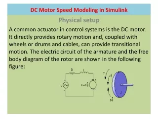
DC Motor Speed Modeling in Simulink Physical setup A common actuator in control systems is the DC motor. It directly provides rotary motion and, coupled with wheels or drums and cables, can provide transitional motion. The electric circuit of the armature and the free body diagram of the rotor are shown in the following figure:
For this example, we will assume the following values for the physical parameters. • moment of inertia of the rotor (J) = 0.01 kg. kg.m2/s2 • damping ratio of the mechanical system (b) = 0.1 Nms • electromotive force constant (K=Ke=Kt) = 0.01 Nm/Amp • electric resistance (R) = 1 ohm • electric inductance (L) = 0.5 H • input (V): Source Voltage • output (theta): position of shaft • The rotor and shaft are assumed to be rigid
The motor torque, T, is related to the armature current, i, by a constant factor Kt. The back emf, e, is also related to the rotational velocity. These two parameters are described by the following equations: In SI units (which we will use), Kt (armature constant) is equal toKe (motor constant).
Next, we will start to model both Newton's law and Kirchoff's law. These laws applied to the motor system give the following equations: • The angular acceleration is equal to 1/J multiplied by the sum of two terms (one +, one -.). Similarly, the derivative of current is equal to 1/L multiplied by the sum of three terms (one +, two -).
Building the Model • This system will be modelled by summing the torques acting on the rotor wheel (inertia toques) and integrating the acceleration to give the velocity. • Also, Kirchoff's laws will be applied to the armature circuit. Open Simulink and open a new model window. First, we will model the integrals of the rotational acceleration and of the rate of change of armature current.
Simulation Procedures • Insert an Integrator block (from the Linear block library) and draw lines to and from its input and output terminals. Label the input line "d2/dt2(theta)" and the output line "d/dt (theta)" as shown below. Insert another Integrator block above the previous one and draw lines to and from its input and output terminals. Label the input line .d/dt(i) and the output line "i".
Simulation procedures ..continued • Insert two Gain blocks, (from the Linear block library) one attached to each of the integrators. • Edit the gain block corresponding to angular acceleration by double-clicking it and changing its value to "1/J". • Change the label of this Gain block to "inertia" by clicking on the word "Gain" underneath the block. • Similarly, edit the other Gain's value to "1/L" and it's label to Inductance. • Insert two Sum blocks (from the Linear block library), one attached by a line to each of the Gain blocks. • Edit the signs of the Sum block corresponding to rotation to "+-" since one term is positive and one is negative. • Edit the signs of the other Sum block to "-+-" to represent the signs of the terms in Kirchoff's equation.
Now, we will add in the torques which are represented in Newton's equation. First, we will add in the damping torque: Insert a gain block below the inertia block, select it by single-clicking on it, and select Flip from the Format menu (or type Ctrl-F) to flip it left-to-right. Set the gain value to "b" and rename this block to "damping".
Tap a line (hold Ctrl while drawing) off the rotational integrator's output and connect it to the input of the damping gain block. • Draw a line from the damping gain output to the negative input of the rotational Sum block. Next, we will add in the torque from the armature. • Insert a gain block attached to the positive input of the rotational Sum block with a line. • Edit it's value to "K" to represent the motor constant and Label it "Kt". • Continue drawing the line leading from the current integrator and connect it to the Kt gain block. The diagram looks like this:
Adding the Voltage Terms Now, we will add in the voltage terms which are represented in Kirchoff's equation. First, we will add in the voltage drop across the coil resistance. • Insert a gain block above the inductance block, and flip it left-to-right. • Set the gain value to "R" and rename this block to "Resistance". • Tap a line (hold Ctrl while drawing) off the current integrator's output and connect it to the input of the resistance gain block. • Draw a line from the resistance gain output to the upper negative input of the current equation Sum block.
Adding the back emf Next, we will add in the back emf from the motor. • Insert a gain block attached to the other negative input of the current Sum block with a line. • Edit it's value to "K" to represent the motor constant and Label it "Ke". • Tap a line off the rotational integrator output and connect it to the (Ke) gain block. Now the diagram looks like this:
Adding the Control Input ‘V’ • The third voltage term in the Kirchoff equation is the control input, V. We will apply a step input. • Insert a Step block (from the Sources block library) and connect it with a line to the positive input of the current Sum block. • To view the output speed, insert a Scope (from the Sinks block library) connected to the output of the rotational integrator. • To provide a appropriate unit step input at t=0, double-click the Step block and set the Step Time to "0". The final model looks like the following:
Open-loop response • To simulate this system, first, an appropriate simulation time must be set. Select Parameters from the Simulation menu and enter "3" in the Stop Time field. 3 seconds is long enough to view the open-loop response. • The physical parameters must now be set. Run the following commands at the MATLAB prompt: • J=0.01; b=0.1; K=0.01; R=1; L=0.5; (or save in an ‘m-file’) • Run the simulation (Ctrl-t or Start on the Simulation menu). When the simulation is finished, double-click on the scope and hit its auto-scale button. You should see the following output.
Implementing Lag Compensator Control • In the motor speed control root locus example a Lag Compensator was designed with the following transfer function. • To implement this in Simulink, we will contain the open-loop system from earlier in this page in a Subsystem block. • Create a new model window in Simulink. • Drag a Subsystem block from the Connections block library into your new model window.