Mass Transfer and Diffusion
Mass Transfer and Diffusion. Mass transfer is the net movement of a component in a mixture from one location to another location where the component exists at a different concentration . ~Mass transfer takes place between two phase across an interface.

Mass Transfer and Diffusion
E N D
Presentation Transcript
Mass Transfer and Diffusion Mass transfer is the net movement of a component in a mixture from one location to another location where the component exists at a different concentration. ~Mass transfer takes place between two phase across an interface. absorption by a liquid of a solute from a gas involves mass transfer of the solute through the gas to the gas-liquid interface, across the interface, and into the liquid. ~Mass transfer models are used to describe processes such as the passage of a species through a gas to the outer surface of a porous adsorbent particles and into the pore of the adsorbent, where the species is adsorbed on the porous surface. ~Mass transfer is also the selective permeation through a nonporous polymeric material of a component of a gas mixture. ~Mass transfer is not the flow of a fluid through a pipe, however, mass transfer might be superimposed on that flow. ~Mass transfer is not the flow of solids on a conveyor belt.
Mass transfer occurs by three basic mechanisms: (1)molecular diffusion by random and spontaneous microscopic movement of individual molecules in a gas, liquid, or solid as result of thermal motion. (2)eddy (turbulent) diffusion by random macroscopic fluid motion. (3)When a net flow occurs in one of these directions, the total rate of mass transfer of individual species is increased or decreased by this bulk flow or convention effect. ~Molecular and/or eddy diffusion frequently involves the movement of different species in opposing directions. ~Molecular diffusion is extremely slow, whereas eddy diffusion, when it occurs, is orders of magnitude more rapid. ~Molecular diffusion occurs in solids and in fluids that are stagnant or in laminar or turbulent motion. ~Eddy diffusion occurs in fluids in turbulent motion. ~When both molecular diffusion and eddy diffusion occur, they take place in parallel and are additive, furthermore, they take place because of the same concentration difference (gradient).
If Ni is the molar flux of species i with mole fraction xi, and N is the total molar flux, with both fluxes in moles per unit time per unit area in a direction perpendicular to a stationary plane across which mass transfer occurs, then Each term in Eq. (*) is positive or negative depending on the direction of the flux relative to the direction selected as positive. When the molecular and eddy diffusion fluxes are in one direction and N is in the opposite direction, even though a concentration difference or gradient of i exists, the net mass transfer flux, Ni, of i can be zero.
Steady-State Ordinary Molecular Diffusion ~Mass transfer by ordinary molecular diffusion occurs because of a concentration difference or gradient; that is, a species diffuses in the direction of decreasing concentration. ~The mass transfer rate is proportional to the area normal to the direction of mass transfer and not to the volume of the mixture. Thus, the rate can be expressed as a flux. ~Mass transfer stops when the concentration is uniform. Fick’s Law of diffusion JAz is the molar flux of A by ordinary molecular diffusion relative to the molar average velocity of the mixture in positive z direction, DAB is the mutual diffusion coefficient of A in B, and dcA/dz is the concentration gradient of A, which is negative in the direction of ordinary molecular diffusion. alternative form If the gas, liquid or solid mixture through which diffusion occurs is isotropic, then value of DAB is independent of direction. The diffusion coefficient is also referred to as the diffusivity and the mass diffusivity (to distinguish it from thermal and momentum diffusivities)
Velocities in Mass Transfer The molar average velocity of the mixture, vM, relative to stationary coordinates is given for a binary mixture as Similarly, the velocity of species i, defined in terms of Ni, is relative to stationary coordinates: Combining Eqs. (*) and (**) with xi=ci/c gives Alternatively, species diffusion velocities, viD, defined in terms of Ji, are relative to the molar average velocity and are defined as the difference between the species velocity and the molar average velocity for the mixture:
From Eq (***), the total species velocity is Combining Eqs. (**) and (****), ni is the molar flow rate in moles per unit time, A is the mass transfer area, the first terms on the right-hand sides are the fluxes resulting from bulk flow, and the second terms on the right-hand sides are the ordinary molecular diffusion fluxes. bulk flow molecular diffusion Two limiting cases are important: 1. Equimolar counterdiffusion (EMD) 2. Unimolecular diffusion (UMD)
Equimolar Counterdiffusion (EMD) The molar fluxes of A and B are equal, but opposite in direction; thus, the total concentration, pressure, and temperature are constant and the mole fraction are maintained constant (but different) at two sides of a stagnant film between z1 and z2. This equality of diffusion coefficients is always true in a binary system of constant molar density.
Example 3.1 Two bulbs are connected by a straight tube, 0.001 m in diameter and 0.15 m in length. Initially the bulb at end 1 contains N2 and the bulb at end 2 contains H2. The pressure and temperature are maintained constant at 25 C and 1 atm. At a certain time after allowing diffusion to occur between the two bulbs, the nitrogen content of the gas at end 1 of the tube is 80 mol% and at end 2 is 25 mol%. If the binary diffusion coefficient is 0.784 cm2/s, determine: (a) The rates and directions of mass transfer of hydrogen and nitrogen in mol/s (b) The species velocities relative to stationary coordinates in cm/s
Unimolecular Diffusion (UMD) Mass transfer of component A occurs through stagnant component B. Thus, The log mean (LM) of (1-xA) at the two ends of the stagnant layer is
Example 3.2 As shown in Figure 3.2, an open beaker, 6 cm in height, is filled with liquid benzene at 25 C to within 0.5 cm of the top. A gentle breeze of dry air at 25 C and 1 atm is blown by a fan across the mouth of the beaker so that evaporated benzene is carried away by convection after it transfers through a stagnant air layer in the beaker. The vapor pressure of benzene at 25 C is 0.131 atm. The mutual diffusion coefficient for benzene in air at 25 C and 1 atm is 0.0905 cm2/s. Compute: (a) The initial rate of evaporation of benzene as a molar flux in mol/cm2-s (b) The initial mole fraction profile in the stagnant layer (c) The initial fractions of the mass transfer fluxes due to molecular diffusion (d) The initial diffusion velocities, and the species velocities (relative to stationary coordinates) in the stagnant layer (e) The time in hours for the benzene level in the beaker to drop 2 cm from the initial level if the specific gravity of liquid benzene is 0.874. Neglect the accumulation of benzene and air in the stagnant layer as it increase in height.
Diffusion Coefficients Diffusivity in Gas Mixtures ~ Fuller et al. DAB is in cm2/s, P is in atm, T is in K ~Experimental values of binary gas diffusivity at 1 atm and near-ambient temperature range from about 0.1 to 10.0 cm2/s. ~When an experimental diffusivity is available at values T and P that are different from the desired conditions, Eq. (*) indicates that DAB is proportional to T1.75/P, which can be used to obtain the desired value.
Example 3.3 Estimate the diffusion coefficient for the system oxygen (A)/benzene (B) at 38 C and 2 atm using the method of Fuller et al. Solution At 1 atm, the predicted diffusivity is 0.0988 cm2/s, which is about 3% below the experimental of 0.102 cm2/s. The experimental value for 38 C can be extrapolated by the temperature dependency of Eq. (*) to give the following equation at 200 C:
~For binary mixture of light gases, at pressures to about 10 atm, the pressure dependence on diffusivity is adequately predicted by the simple inverse relation, that is, PDAB=a constant for a given temperature and gas mixture. ~At higher pressure, deviation from this relation are handled in a manner somewhat similar to the modification of the ideal gas law by the compressibility factor based on the theorem of corresponding states. ~Takahasi has published a tentative corresponding-states correlation for high pressure, shown in Figure 3.3. ~In the Takahasi plot, DABP/(DABP)LP is given as a function of reduced temperature and pressure, where (DABP)LP is at low pressure where Eq. (*) applies. ~Mixture critical temperature and pressure are molar-average values.
Example 3.4 Estimate the diffusion coefficient for a 25/75 molar mixture of argon and xenon at 200 atm and 378 K. At this temperature and 1 atm, the diffusion coefficient is 0.180 cm2/s. Critical constants are Solution From Figure 3.3, DABP/(DABP)LP is 0.82
Diffusivity in Liquid Mixtures Wilke-Chang equation for small solute molecules when water is the solvent where the units are cm2/s for DAB; cP for the solvent viscosity, B; K for T; and cm3/mol for vA,the liquid molar volume of the solute at its normal boiling point. The parameter B is an association factor for the solvent, which for water is 2.6. vA can be estimated by summing the atomic contributions in Table 3.2, which also lists values of vA for dissolved light gases.
Example 3.5 Use the Wilke-Chang equation to estimate the diffusivity of aniline (A) in a 0.5 mol% aqueous solution at 20 C. At this temperature, the solubility of aniline in water is about 4g/100g of water or 0.77 mol% anile. The experimental diffusivity value for an infinitely dilute mixture is 0.9210-5 cm2/s. Solution This value is about 3% less than the experimental value of an infinite dilute solution of aniline in water. Although Wilke and Chang determined values B for methanol (1.9), ethanol (1.5), and unassociated solvent (1.0), more recent correlation due to Hayduk and Minhas give better agreement with experimental values. For a dilute solution of one normal paraffin (C5 to C32) in another (C5 to C16),
For general nonaqueous solutions, where P is the parachor, which is defined as When the units of the liquid molar volume, v, are cm3/mol and the surface tension, , are g/s2, then the units of the parachor are cm3-g1/4 /s1/2-mol. The following restriction apply to Eq. (*) 1.Solvent viscosity should not exceed 30 cP. 2.For organic acid solutes and solvents other than water, methanol, and butanols, the acid should be treated as a dimer by doubling the values of PA and vA. 3.For a nonpolar solute in monohydroxy alcohols, values of vB and PB should be multiplied by 8B, where the viscosity is in cP.
Normally, at near-ambient conditions, P is treated as a constant, for which an extensive tabulation is available from Quayle, who also provides a group-contribution method for estimating parachors for compound not listed. Table 3.3 gives values of parachors for a number of compounds, while Table 3.4 contains structural contributions for predicting the parachor in the absence of data.
Example 3.6 Estimate the diffusivity of formic acid (A) in benzene (B) at 25 C and infinite diffusion, using the appropriate correlation of Hayduck and Minhas. The experimental value is 2.2810-5 cm2/s. Solution However, because formic acid is an organic acid, PA is doubled to 187.4. which is within 6% of the experimental value.
~The Wilke-Chang equations predict an inverse dependence of viscosity with liquid diffusivity. The Hayduk-Minhas equations predict somewhat smaller dependence of viscosity. ~From data covering several orders of magnitude variation of viscosity, the liquid diffusivity is found to vary inversely with the viscosity raised to an exponent closer to 0.5 than to 1.0. The Wilke-Chang equation also predict that DABB/T is a constant over a narrow temperature range. ~Because B decreases exponentially with temperature, DAB is predicted to increase exponentially with temperature. Over a wide temperature range, it is preferable to express the effect of temperature on DAB by an Arrhenius-type expression, where, typically the activation energy for liquid diffusion, E, is no greater than 6,000 cal/mol.
~Liquid diffusion coefficients for a solute in a dilute binary system range from about 10-6 to 10-4 cm2/s for solutes of molecular weight up to 200 and solvents with viscosity up to about 10 cP. ~Thus, liquid diffusivities are five orders of magnitude less than diffusivities for binary gas mixtures at 1 atm. ~However, diffusion rates in liquids are not necessarily five order lower than in gases because the product of the concentration (molar density) and the diffusivity determines the rate of diffusion for a given concentration gradient in mole fraction. ~At 1 atm, the molar density of a liquid is three times that of a gas and, thus, the diffusion rate in liquids is only two orders of magnitude lower than in gases at 1 atm.
One-Dimensional Steady-State and Unsteady-State Molecular Diffusion In terms of mass transfer rate by diffusion only across the plane, For steady-state, one-dimensional diffusion, with constant DAB, Eq. (*) can be integrated for various geometries, the most common results being analogous to heat conduction. 1. Plane wall with a thickness, z2-z1: 2. Hollow cylindrical of inner radius r1 and outer radius r2, with diffusion in the radial direction outward: ALM=log mean of the area 2rL at r1 and r2 L=length of the hollow cylinder 3. Spherical shell of inner radius r1 and outer radius r2, with diffusion in the radial direction outward: AGM=geometric mean of the area 4r2 at r1 and r2
Consider the one-dimensional diffusion through species B of species A through a differential control volume with diffusion in the z direction only, as shown in Figure 3.5. Assume constant total concentration, c=cA+cB, constant diffusivity, and negligible bulk flow, Fick’s second law for one-dimensional diffusion The more general for, for three-dimensional rectangular coordinates, is For one-dimensional diffusion in the radial direction only, for cylindrical and spherical coordinates, Fick’s second law becomes, respectively,
Consider the semiinfinite medium shown in Figure 3.6, which extends in the z direction from z=0 to z=. The x and y coordinate extend form - to +, but are not of interest because diffusion takes place only in the z direction. B.C cA=cA0 for t=0 cA=cAs for z=0 cA=cA0 for z= as the penetration depth
Example 3.11 Determine how long it will take for the dimensionless concentration change, =(cA-cA0)/ cAs-cA0), to reach 0.01 at a depth z=1 m in a semiinfinite medium, which is initially at a solute concentration cA0, after the surface concentration at z=0 increases to cAs, for diffusivities representative of a solute diffusing through a gas, a liquid, and a solid. Solution For a gas, assume DAB=0.1 cm2/s. We know that z=1 m=100 cm. For a liquid (DAB=110-5), t=2.39 year For a solid (DAB=110-9), t=239 centuries These results show that molecular diffusion is very slow, especially in liquids and solids. In liquids and gases, the rate of mass transfer can be greatly increased by agitation to induce turbulent motion. For solids, it is best to reduce the diffusion path to as small a dimension as possible.
Consider a rectangular parallelepiped medium of finite thickness 2a in the z direction, and either infinitely long dimensions in the y and x directions or finite lengths of 2b and 2c, respectively, in those directions. Assume that in Figure 3.7a the edges parallel to the z direction are sealed, so diffusion occurs only in the z direction and initially the concentration of the solute in the medium is uniform at cA0. B.C cA=cA0 for t=0 cA=cAs for z=a, t=0 cA/z=0 for z=0
When the edges of the slab in Figure 3.7a are not sealed, the method of Newman can be used to determine concentration changes within the slab. In this method, E or Eavg is given in terms of the E values from the solution of Fick’s second law for each of the coordinate directions by
Example 3.12 A piece of lumber, measuring 51020 cm, initially contains 20 wt% moisture. At time 0, all six faces are brought to an equilibrium moisture content of 2 wt%. Diffusivities for moisture at 25 C are 210-5 cm2/s in the axial (z) direction along the fibers and 410-6 cm2/s in the two directions perpendicular to the fibers. Calculate the time in hours for the average moisture content to drop to 5 wt% at 25 C. At that time, determine the moisture content at the center of the piece of lumber.