Reinforcement learning
Reinforcement learning. Regular MDP Given: Transition model P(s’ | s, a) Reward function R(s) Find: Policy (s) Reinforcement learning Transition model and reward function initially unknown Still need to find the right policy “Learn by doing”. Reinforcement learning: Basic scheme.

Reinforcement learning
E N D
Presentation Transcript
Reinforcement learning • Regular MDP • Given: • Transition model P(s’ | s, a) • Reward function R(s) • Find: • Policy (s) • Reinforcement learning • Transition model and reward function initially unknown • Still need to find the right policy • “Learn by doing”
Reinforcement learning: Basic scheme • In each time step: • Take some action • Observe the outcome of the action: successor state and reward • Update some internal representation of the environment and policy • If you reach a terminal state, just start over (each pass through the environment is called a trial) • Why is this called reinforcement learning?
Applications of reinforcement learning • Backgammon http://www.research.ibm.com/massive/tdl.html http://en.wikipedia.org/wiki/TD-Gammon
Applications of reinforcement learning • Learning a fast gait for Aibos Initial gait Learned gait Policy Gradient Reinforcement Learning for Fast Quadrupedal LocomotionNate Kohl and Peter Stone.IEEE International Conference on Robotics and Automation, 2004.
Applications of reinforcement learning • Stanford autonomous helicopter
Reinforcement learning strategies • Model-based • Learn the model of the MDP (transition probabilities and rewards) and try to solve the MDP concurrently • Model-free • Learn how to act without explicitly learning the transition probabilities P(s’ | s, a) • Q-learning: learn an action-utility function Q(s,a) that tells us the value of doing action a in state s
Model-based reinforcement learning • Basic idea: try to learn the model of the MDP (transition probabilities and rewards) and learn how to act (solve the MDP) simultaneously • Learning the model: • Keep track of how many times state s’ follows state s when you take action a and update the transition probability P(s’ | s, a) according to the relative frequencies • Keep track of the rewards R(s) • Learning how to act: • Estimate the utilities U(s) using Bellman’s equations • Choose the action that maximizes expected future utility:
Model-based reinforcement learning • Learning how to act: • Estimate the utilities U(s) using Bellman’s equations • Choose the action that maximizes expected future utility given the model of the environment we’ve experienced through our actions so far: • Is there any problem with this “greedy” approach?
Exploration vs. exploitation • Exploration: take a new action with unknown consequences • Pros: • Get a more accurate model of the environment • Discover higher-reward states than the ones found so far • Cons: • When you’re exploring, you’re not maximizing your utility • Something bad might happen • Exploitation: go with the best strategy found so far • Pros: • Maximize reward as reflected in the current utility estimates • Avoid bad stuff • Cons: • Might also prevent you from discovering the true optimal strategy
Incorporating exploration • Idea: explore more in the beginning, become more and more greedy over time • Standard (“greedy”) selection of optimal action: • Modified strategy: Number of times we’ve taken action a’ in state s exploration function (optimistic reward estimate)
Model-free reinforcement learning • Idea: learn how to act without explicitly learning the transition probabilities P(s’ | s, a) • Q-learning: learn an action-utility function Q(s,a) that tells us the value of doing action a in state s • Relationship between Q-values and utilities:
Model-free reinforcement learning • Q-learning: learn an action-utility function Q(s,a) that tells us the value of doing action a in state s • Equilibrium constraint on Q values: • Problem: we don’t know (and don’t want to learn) P(s’ | s, a)
Temporal difference (TD) learning • Equilibrium constraint on Q values: • Temporal difference (TD) update: • Pretend that the currently observed transition (s,a,s’) is the only possible outcome and adjust the Q values towards the “local equilibrium”
Temporal difference (TD) learning • At each time step t • From current state s, select an action a: • Get the successor state s’ • Perform the TD update: Exploration function Number of times we’ve taken action a’ from state s Learning rate Should start at 1 and decay as O(1/t) e.g., (t) = 60/(59 + t)
Function approximation • So far, we’ve assumed a lookup table representation for utility function U(s) or action-utility function Q(s,a) • But what if the state space is really large or continuous? • Alternative idea: approximate the utility function as a weighted linear combination of features: • RL algorithms can be modified to estimate these weights • Recall: features for designing evaluation functions in games • Benefits: • Can handle very large state spaces (games), continuous state spaces (robot control) • Can generalize to previously unseen states

