Position Control using Lead Compensators
Position Control using Lead Compensators. Bill Barraclough. Sheffield Hallam University. Technology considered. A small d.c. motor actually to drive the system Torque (and therefore acceleration) depends on applied voltage Back e.m.f. of the motor means the T.F. is of the form K/[s(1 + Ts)]


Position Control using Lead Compensators
E N D
Presentation Transcript
Position Control using Lead Compensators Bill Barraclough Sheffield Hallam University
Technology considered • A small d.c. motor actually to drive the system • Torque (and therefore acceleration) depends on applied voltage • Back e.m.f. of the motor means the T.F. is of the form K/[s(1 + Ts)] • So it inherently contains integration !
Possible Controllers • Proportional + Derivative (Stability problems will arise if we include integration) • Velocity feedback using a tachogenerator • Lead Compensator • We will concentrate on the lead compensator but we will also mention the other possibilities
The lead compensator • These controllers often provide good performance without some of the drawbacks of the p.i.d. • We will obtain the transfer function of a suitable lead compensator for a small d.c. motor used to control position ... • ... and produce a digital version.
The Motor • We will base the work on a motor type which we have in the laboratory ... • ... and on which you will have the opportunity to try out the resulting controllers !
The Lead Compensator • Its transfer function (and that of the lag compensator) is of the form
The Motor • The laboratory motors have a transfer function approximately
The Procedure • Obtain the TF in “s” of the lead compensator • Digitise it • Implement it !
Two Approaches • Decide to replace the motor’s “pole” by a faster one. This determines “a” ... • ... and use trial and error to find “K” and “b”. • Or decide the closed-loop T.F. we require and deduce the controller T.F. needed to achieve it.
Method 1: “Trial and Error” • Controller transfer function:
MATLAB/SIMULINK to the rescue! • Use of MATLAB and SIMULINK suggested that good performance would result from the following controller:
We have two methods of digitising this T.F. • The “simple” method • The “Tustin” method
Which is better ? • The simple method is easier algebraically • but ... • The Tustin method leads to a controller which performs more nearly like the analogue version.
The Simple Method • We will do the conversion by the simple method using an interval Ts of 0.1 s. • 1.33(s+2.5)/(s+7) becomes ... • 1.33[(1-z-1)/0.1 + 2.5]/[(1-z-1)/0.1 + 7] • which by algebra gives • (0.9782 - 0.7824z-1)/(1 - 0.5882z-1)
The Tustin Method • Now the sum becomes (since 2/Ts = 20) • 1.33[20(1-z-1)/(1+z-1)+2.5]/[20(1-z-1)/(1+z-1) + 7] • giving by unreliable Barraclough mathematics • (1.1085 - 0.8619z-1)/(1 - 0.4815z-1)
How do the controllers perform ? • Both digital versions have slightly more overshoot than the analogue version. • The Tustin one is nearer to the analogue version than is the “simple” one. • Both digital versions give a reasonably good performance.
Designing for a particular closed-loop performance • Suppose we decide we require an undamped natural frequency of 5 rad/s ... • ... and a damping ratio of 0.8. • This means that the closed-loop transfer function needs to be • 25/(s2 + 8s + 25)
The required controller T.F. ? • We have: • So forward path = D(s) x G(s) .. • and the CLTF is D(s)G(s)/[1 + D(s)G(s)] D(s) G(s) + _
The sum continues ... • This means that • D(s)G(s)/[1 + D(s)G(s)] = 25/(s2 + 8s + 25) • and as G(s) = 12/[s(s + 2.5)] • we will show that • D(s) must be 2.08(s + 2.5)/(s + 8) • to produce the required performance.
Your turn ! • If we use a sampling interval of 0.1 s again • What will the digitised transfer functions be • using the simple method ... • ... and the Tustin method ? • We can check the Tustin one by MATLAB • using the “c2dm” command.
“Your Turn” continued • The syntax is • [nd,dd]=c2dm(num,den,ts,’tustin’) • num and den represent the T.F. in s • ts is the sampling interval • nd and dd represent the T.F. in z.
Summary • Lead compensators are often useful in position control systems using a d.c. motor • with a “Type 1” transfer function. • We have examined two methods of doing the digitisation. • The Tustin method gives the best approximation to the analogue performance for a given sampling interval.