Routing
Routing. An Engineering Approach to Computer Networking. What is it?. Process of finding a path from a source to every destination in the network Suppose you want to connect to Antarctica from your desktop what route should you take? does a shorter route exist?

Routing
E N D
Presentation Transcript
Routing An Engineering Approach to Computer Networking
What is it? • Process of finding a path from a source to every destination in the network • Suppose you want to connect to Antarctica from your desktop • what route should you take? • does a shorter route exist? • what if a link along the route goes down? • what if you’re on a mobile wireless link? • Routing deals with these types of issues
Basics • A routing protocol sets up a routing table in routers and switch controllers • A node makes a local choice depending on global topology: this is the fundamentalproblem
Key problem • How to make correct local decisions? • each router must know something about global state • Global state • inherently large • dynamic • hard to collect • A routing protocol must intelligently summarize relevant information
Requirements • Minimize routing table space • fast to look up • less to exchange • Minimize number and frequency of control messages • Robustness: avoid • black holes • loops • oscillations • Use optimal path
Choices • Centralized vs. distributed routing • centralized is simpler, but prone to failure and congestion • Source-based vs. hop-by-hop • how much is in packet header? • Intermediate: loose source route • Stochastic vs. deterministic • stochastic spreads load, avoiding oscillations, but misorders • Single vs. multiple path • primary and alternative paths (compare with stochastic) • State-dependent vs. state-independent • do routes depend on current network state (e.g. delay)
Outline • Routing in telephone networks • Distance-vector routing • Link-state routing • Choosing link costs • Hierarchical routing • Internet routing protocols • Routing within a broadcast LAN • Multicast routing • Routing with policy constraints • Routing for mobile hosts
Telephone network topology • 3-level hierarchy, with a fully-connected core • AT&T: 135 core switches with nearly 5 million circuits • LECs may connect to multiple cores
Routing algorithm • If endpoints are within same CO, directly connect • If call is between COs in same LEC, use one-hop path between COs • Otherwise send call to one of the cores • Only major decision is at toll switch • one-hop or two-hop path to the destination toll switch • (why don’t we need longer paths?) • Essence of problem • which two-hop path to use if one-hop path is full
Features of telephone network routing • Stable load • can predict pairwise load throughout the day • can choose optimal routes in advance • Extremely reliable switches • downtime is less than a few minutes per year • can assume that a chosen route is available • can’t do this in the Internet • Single organization controls entire core • can collect global statistics and implement global changes • Very highly connected network • Connections require resources (but all need the same)
Statistics • Posson call arrival (independence assumption) • Exponential call “holding” time (length!) • Goal:- Minimise Call “Blocking” (aka “loss”) Probability subject to minimise cost of network
The cost of simplicity • Simplicity of routing a historical necessity • But requires • reliability in every component • logically fully-connected core • Can we build an alternative that has same features as the telephone network, but is cheaper because it uses more sophisticated routing? • Yes: that is one of the motivations for ATM • But 80% of the cost is in the local loop • not affected by changes in core routing • Moreover, many of the software systems assume topology • too expensive to change them
Dynamic nonhierarchical routing (DNHR) • Simplest core routing protocol • accept call if one-hop path is available, else drop • DNHR • divides day into around 10-periods • in each period, each toll switch is assigned a primary one-hop path and a list of alternatives • can overflow to alternative if needed • drop only if all alternate paths are busy • crankback • Problems • does not work well if actual traffic differs from prediction
Metastability • Burst of activity can cause network to enter metastable state • high blocking probability even with a low load • Removed by trunk reservation • prevents spilled traffic from taking over direct path
Trunk status map routing (TSMR) • DNHR measures traffic once a week • TSMR updates measurements once an hour or so • only if it changes “significantly” • List of alternative paths is more up to date
Real-time network routing • No centralized control • Each toll switch maintains a list of lightly loaded links • Intersection of source and destination lists gives set of lightly loaded paths • Example • At A, list is C, D, E => links AC, AD, AE lightly loaded • At B, list is D, F, G => links BD, BF, BG lightly loaded • A asks B for its list • Intersection = D => AD and BD lightly loaded => ADB lightly loaded => it is a good alternative path • Very effective in practice: only about a couple of calls blocked in core out of about 250 million calls attempted every day
DynamicAlternativeRouting Very simple idea, but can be shown to provide optimal routes at very low complexity… November 2001 Dynamic Alternative Routing 17
Underlying Network Properties Fully connected network Underlying network is a trunk network Relatively small number of nodes In 1986, the trunk network of British Telecom had only 50 nodes Any algorithm with polynomial running time works fine Stochastic traffic Low variance when the link is nearly saturated November 2001 Dynamic Alternative Routing 18
Dynamic Alternative Routing Proposed by F.P. Kelly, R. Gibbens at British Telecom (well, Cambridge, Really:) Whenever the link (i, j) is saturated, use an alternative node (tandem) Q. How to choose tandem? Ci,j i j k November 2001 Dynamic Alternative Routing 19
Fixed Tandem For any pair of nodes (i, j) we assign a fixed node k as tandem Needs careful traffic analysis and reprogramming Inflexible during breakdowns and unexpected traffic at tandem November 2001 Dynamic Alternative Routing 20
Sticky Random Tandem If there is no free circuit along (i, j), a new call is routed through a randomly chosen tandem k k is the tandem as long as it does not fail If k fails for a call, the call is lost and a new tandem is selected November 2001 Dynamic Alternative Routing 21
Sticky Random Tandem Decentralized and flexible No fancy pre-analysis of traffic required Most of the time friendly tandems are used: pk(i, j): proportion of calls between i and j which go through k qk(i, j): proportion of calls that are blocked pa(i, j)qa(i, j) = pb(i, j)qb(i, j) We may assign different frequencies to different tandems November 2001 Dynamic Alternative Routing 22
Trunk Reservation A tandem k accepts to forward calls if it has free capacity more than R • Unselfishness towards one’s friends is good up to a point!!! • We need to penalize two link calls, at least when the lines are very busy! i j k November 2001 Dynamic Alternative Routing 23
Trunk Reservation November 2001 Dynamic Alternative Routing 24
Bounds: Erlang’s Bound • A node connected to C circuits • Arrival: Poisson with mean v • The expected value of blocking: November 2001 Dynamic Alternative Routing 25
Max-flow Bound Capacity of (i, j): Cij Mean load on (i, j): vij where f is: Cij i j k November 2001 Dynamic Alternative Routing 26
Trunk Reservation November 2001 Dynamic Alternative Routing 27
Traffic, Capacity Mismatch • Traffic > Capacity for some links • Can we always find a feasible set of tandems? • Red links: saturated links • White links: not saturated • Good triangle: one red, two white links November 2001 Dynamic Alternative Routing 28
Greedy Algorithm Success! Fail Tk+1 a. No red links b. Red link and a good triangle • Add good triangle to the list c. Red link and no good triangle Success! T1 Tk T2 November 2001 Dynamic Alternative Routing 29
Greedy Algorithm Success! Fail Tk+1 a. No red links b. Red link and a good triangle • Add good triangle to the list c. Red link and no good triangle Success! For any p < 1/3, the greedy algorithm is successful with probability approaching 1. T1 Tk T2 November 2001 Dynamic Alternative Routing 30
Extensions to DAR n-link paths Too much resources consumed, little benefit Multiple alternatives M attempts before rejecting a call Least-busy alternative Repacking A call in progress can be rerouted November 2001 Dynamic Alternative Routing 31
Comparison of Extensions November 2001 Dynamic Alternative Routing 32
Features of Internet Routing • Packets, not circuits ( • E.g. timescales can be much shorter • Topology complicated/heterogeneous • Many (10,000 ++) providers • Traffic sources bursty • Traffic matrix unpredictable • E.g. Not distance constrained • Goal: maximise throughput, subject to min delay and cost (and energy?)
Internet Routing Model • 2 key features: • Dynamic routing • Intra- and Inter-AS routing, AS = locus of admin control • Internet organized as “autonomous systems” (AS). • AS is internally connected • Interior Gateway Protocols (IGPs) within AS. • Eg: RIP, OSPF, HELLO • Exterior Gateway Protocols (EGPs) for AS to AS routing. • Eg: EGP, BGP-4
Requirements for Intra-AS Routing • Should scale for the size of an AS. • Low end: 10s of routers (small enterprise) • High end: 1000s of routers (large ISP) • Different requirements on routing convergence after topology changes • Low end: can tolerate some connectivity disruptions • High end: fast convergence essential to business (making money on transport) • Operational/Admin/Management (OAM) Complexity • Low end: simple, self-configuring • High end: Self-configuring, but operator hooks for control • Traffic engineering capabilities: high end only
Requirements for Inter-AS Routing • Should scale for the size of the global Internet. • Focus on reachability, not optimality • Use address aggregation techniques to minimize core routing table sizes and associated control traffic • At the same time, it should allow flexibility in topological structure (eg: don’t restrict to trees etc) • Allow policy-based routing between autonomous systems • Policy refers to arbitrary preference among a menu of available options (based upon options’ attributes) • In the case of routing, options include advertised AS-level routes to address prefixes • Fully distributed routing (as opposed to a signaled approach) is the only possibility. • Extensible to meet the demands for newer policies.
c b b c a network layer inter-AS, intra-AS routing in gateway A.c link layer physical layer A.c A.a C.b B.a Intra-AS and Inter-AS routing • Gateways: • perform inter-AS routing amongst themselves • perform intra-AS routers with other routers in their AS b a a C B d A
Inter-AS routing between A and B b c a a C b B b a c d Host h1 A A.a A.c C.b B.a Intra-AS and Inter-AS routing: Example Host h2 Intra-AS routing within AS B Intra-AS routing within AS A
Basic Dynamic Routing Methods • Source-based: source gets a map of the network, • source finds route, and either • signals the route-setup (eg: ATM approach) • encodes the route into packets (inefficient) • Link state routing: per-link information • Get map of network (in terms of link states) at all nodes and find next-hops locally. • Maps consistent => next-hops consistent • Distance vector:per-node information • At every node, set up distance signposts to destination nodes (a vector) • Setup this by peeking at neighbors’ signposts.
Where are we? • Routing vs Forwarding • Forwarding table vs Forwarding in simple topologies • Routers vs Bridges: review • Routing Problem • Telephony vs Internet Routing • Source-based vs Fully distributed Routing • Distance vector vs Link state routing • Bellman Ford and Dijkstra Algorithms • Addressing and Routing: Scalability
DV & LS: consistency criterion • The subset of a shortest path is also the shortest path between the two intermediate nodes. • Corollary: • If the shortest path from node i to node j, with distance D(i,j) passes through neighbor k, with link cost c(i,k), then: D(i,j) = c(i,k) + D(k,j) j D(k,j) i c(i,k) k
Distance Vector DV = Set (vector) of Signposts, one for each destination
1 1 7 A A A D D E B B E B E C C 7 7 2 8 8 1 1 1 2 2 Example network A’s 1-hop view (After 1st iteration) A’s 2-hop view (After 2nd Iteration) Distance Vector (DV) Approach Consistency Condition: D(i,j) = c(i,k) + D(k,j) • The DV (Bellman-Ford) algorithm evaluates this recursion iteratively. • In the mth iteration, the consistency criterion holds, assuming that each node sees all nodes and links m-hops (or smaller) away from it (i.e. an m-hop view)
Distance Vector (DV)… • Initial distance values (iteration 1): • D(i,i) = 0 ; • D(i,k) = c(i,k) if k is a neighbor (i.e. k is one-hop away); and • D(i,j) = INFINITY for all other non-neighbors j. • Note that the set of values D(i,*) is a distance vector at node i. • The algorithm also maintains a next-hop value (forwarding table) for every destination j, initialized as: • next-hop(i) = i; • next-hop(k) = k if k is a neighbor, and • next-hop(j) = UNKNOWN if j is a non-neighbor.
Distance Vector (DV)… • After every iteration each node iexchanges its distance vectors D(i,*) with its immediate neighbors. • For any neighbor k, if c(i,k) + D(k,j) < D(i,j), then: • D(i,j) = c(i,k) + D(k,j) • next-hop(j) = k • After each iteration, the consistency criterion is met • After miterations, each node knows the shortest path possible to any other node which is m hops or less. • I.e. each node has an m-hop view of the network. • The algorithm converges (self-terminating) in O(d) iterations: d is the maximum diameter of the network.
1 1 7 A A A D D E B B E B E C C 7 7 2 8 8 1 1 1 2 2 Example network A’s 1-hop view (After 1st iteration) A’s 2-hop view (After 2nd Iteration) Distance Vector (DV) Example • A’s distance vector D(A,*): • After Iteration 1 is: [0, 7, INFINITY, INFINITY, 1] • After Iteration 2 is: [0, 7, 8, 3, 1] • After Iteration 3 is: [0, 7, 5, 3, 1] • After Iteration 4 is: [0, 6, 5, 3, 1]
1 4 1 50 X Z Y Distance Vector: link cost changes Link cost changes: node detects local link cost change updates distance table if cost change in least cost path, notify neighbors “good news travels fast” algorithm terminates
60 4 1 50 X Z Y Distance Vector: link cost changes Link cost changes: good news travels fast bad news travels slow - “count to infinity” problem! algo goes on!
60 4 1 50 X Z Y Distance Vector: poisoned reverse If Z routes through Y to get to X : Z tells Y its (Z’s) distance to X is infinite (so Y won’t route to X via Z) At Time 0, DV(Z) as seen by Y is [INF INF 0],not[5 1 0] ! algorithm terminates
Link State (LS) Approach • The link state (Dijkstra) approach is iterative, but it pivots around destinations j, and their predecessors k = p(j) • Observe that an alternative version of the consistency condition holds for this case: D(i,j) = D(i,k) + c(k,j) • Each node i collects all link states c(*,*) first and runs the complete Dijkstra algorithm locally. j c(k,j) i D(i,k) k