Download
1 / 76
760 likes | 933 Vues
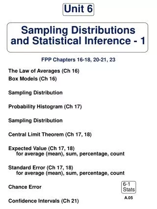
The Law of Averages (Ch 16) Box Models (Ch 16) Sampling Distribution Probability Histogram (Ch 17) Sampling Distribution Central Limit Theorem (Ch 17, 18) Expected Value (Ch 17, 18) for average (mean), sum, percentage, count

E N D
The Law of Averages (Ch 16) Box Models (Ch 16) Sampling Distribution Probability Histogram (Ch 17) Sampling Distribution Central Limit Theorem (Ch 17, 18) Expected Value (Ch 17, 18) for average (mean), sum, percentage, count Standard Error (Ch 17, 18) for average (mean), sum, percentage, count Chance Error Confidence Intervals (Ch 21) Unit 6Sampling Distributionsand Statistical Inference - 1FPP Chapters 16-18, 20-21, 23 A.05
The Law of Averages • Toss a coin 10,000 times. • At each toss we expect 50% to be heads. • At each toss let’s note • the number of heads • the percentage of heads
The Law of Averages With a large number of tosses, the percentage of heads is likely to be close to 50%, although it is not likely to be exactly equal to 50%.
The Law of Averages does NOT say … “The ___________________ team has had such a long string of losses, they are due to get a win. Therefore their chances of winning the next game are greater.” “I have tossed a coin many times, and now have a string of 5 heads. So the chances of getting tails on the next toss must be greater than 50%.”
Number of Heads,Chance Error • Number of heads = • 50% of the number of tosses + • chance error • Can we assess what the chance error is?
Coin toss example • It turns out that • - after 100 tosses, chance error = 5 • - after 10,000 tosses, chance error = 50 • - increasing the number of tosses by 100 times, chance error increases _______ times. • Why does the percentage go to 50%?
Example • We have the choice of tossing a coin 10 times or 100 times. We win if • we get more than 60% heads. • we get more than 40% heads. • we get between 40% and 60% heads. • we get exactly 50% heads. • Should we toss 10 or 100 times?
Baseball series • Team A believes that on any day they have a 60% chance of beating Team B. • They have the option of playing • 1 game, or • best 2 out of 3 • Which format should they choose?
Where we are headed • We want to perform a political survey and randomly sample citizens. • We want to quantify the chance variability of our sample. (We don’t want all to be republican). • We can solve variability questions like these by analogy with drawing from a box.
In practice, what do we really know / not know? Why do we make box models? Making a Box Model In specifying a box model, we would like to know - What numbers go into the box - How many of each kind - How many draws (sample size)
1 2 3 4 5 6 Variability in the box model • Sample 25 tickets with replacement. • Record the sum of the 25 tickets. • 3 2 3 2 6 4 6 5 1 5 6 1 5 3 1 • 3 5 2 4 2 2 6 5 3 4 • Their sum is 89.
Try again • 4 4 6 1 4 1 6 1 5 2 1 4 5 2 1 • 4 5 2 2 5 4 3 3 2 6 • •sum is 83 • 3 2 3 5 1 4 4 6 5 1 2 1 5 2 1 • 2 4 3 4 6 1 6 3 1 3 • sum is 78 • Other tries: 82, 92, 71, 73, 90 • Range is 25 to 150 but we only observed 71 to 92.
Roulette • A roulette wheel has 38 pockets • 18 red numbers • 18 black numbers • 2 green (0 and 00) • We put a dollar on red. What are the chances of winning? • What numbers are in the box?
Net gain • Net gain is the amount that we have won or lost. • Let’s play 10 times… • R R R B G R R B B R • +1 +1 +1 –1 –1 +1 +1 –1 –1 +1 • +1 +2 +3 +2 +1 +2 +3 +2 +1 +2
Which game? • You win if you draw a “1”. • A box has 1 “0” ticket and 9 “1” tickets. • Or • A box has 10 “0” ticket and 90 “1” tickets. • Or • You draw 10 times with replacement. If the sum is 10 then you win.
“The expected value for the sum of draws made at random with replacement from a box” equals the expected value for a sample sum equals A sample sum is likely to be around its expected value, but to be off by a chance error similar in size to the standard error for sum. Expected ValueChapt 17
The standard error for sum, SE(sum), for a random sample of a given sample size is . In FPP, this is . Standard Error for Sum
The sample sum is likely to be around ____________, give or take ____________or so. The expected value for the sum, EV(sum), fills the first blank. The standard error for sum, SE(sum), fills the second blank. Observed values are rarely more than 2 or 3 SE’s away from the expected value. A Sample Sum is Likely ...
The formulas here are for simple random samples. They likely do not apply to other kinds of samples. A Reminder
In Keno, if you bet on one number, if you win you get $2, if you lose you lose $1. The chance of winning is ¼________. What does the box model look like? What is the expected net gain after 100 plays? Example - Keno
In MegaMillions,you pay $1 to play. You select 5 numbers between 1 and 56, and one MegaBall number between 1 and 46. If you match all 5 numbers AND the MegaBall number, you win the jackpot (starts at $12 million). The chance of winning is ¼_____. What does the box model look like? What is the expected net gain after 100 plays? ExampleWashington State Lottery
Today’s jackpot is ___________. Suppose you play 10 times. We want to know about your net gain. What is the relevant box model? Washington State Lotterycontinued
What is the expected net gain if you buy 100 tickets? What does that mean? What is the standard error for your net gain? What does that tell us? Washington State Lotterycontinued
Earlier in the course we displayed data in histograms. Probability histogram • • Probability histograms represent the true (as opposed to the data) chance of an outcome. • Example: rolling a die
Sum of two die 1,000 100 10,000 truth
After rolling 100 times we see that we never rolled a 2. But we know a 2 is possible. After rolling 1,000 times the distribution seems more symmetric After 10,000 the histogram is symmetric. The empirical histogram converges to the true histogram. Empirical vs. truth
There are two counts that may be confused the number of things added together the number of repetitions of the experiment As the number of repetitions increases, the empirical distribution converges to the true histogram. What happens when the number of things added together increases? Caution
“The expected value for the average of draws made at random with replacement from a box” equals the expected value for a sample mean equals A sample average (mean) is likely to be around its expected value, but to be off by a chance error similar in size to the standard error for average. Expected ValueChapt 23
The standard error for average, SE(avg), for a random sample of a given sample size is . In FPP, this is . Standard Error for Average
The sample average is likely to be around __________ _, give or take ____________or so. The expected value for the average, EV(avg), fills the first blank. The standard error for average, SE(avg), fills the second blank. Observed values are rarely more than 2 or 3 SE’s away from the expected value. A Sample Average is Likely ...
The formulas here are for simple random samples. They likely do not apply to other kinds of samples. A Warning
Toss a coin 100 times Probability histogramsand the normal curve Average = 50 SD = 5
• A coin is tossed 100 times. Use the normal curve to estimate the chances of exactly 50 heads (7.96%) between 45 and 55 heads inclusive (72.87%) between 45 and 55 heads exclusive (63.19%) Probability histograms can be difficult to compute but the normal curve is easy. Using the Normal
Assume that the box has tickets 1,9,5,5,5 Drawing from a lopsided box
When drawing • a LARGE sample • at random • with replacement from a box, And computing the sample sum of draws (net gain), the sample count (# heads), the sample average, or the sample percent, the probability histogram will follow a normal curve. = Central Limit Theorem
When the sample size is large enough, to use a normal curve to make probability calculations we simply need the expected value of the sum (This can tell us about the ) the standard error of the sum (This can tell us about the ) Central Limit Theorem
When drawing • a LARGE sample • at random • with replacement from a box, the probability histogram for the sample sum will follow a normal curve. The average of this probability histogram is the EV(sum), and the SD of this probability histogram is SE(sum). Central Limit Theorem
When drawing • a LARGE sample • at random • with replacement from a box, And computing the average of draws, the probability histogram for the sample average (mean) will follow a normal curve. The average of this probability histogram is the EV(avg) = the population mean, and the SD of this probability histogram is SE(avg). Central Limit Theorem
In practice 68% of the time the observed sum will be between expected value 1 SE 95% of the time the observed sum will be between expected value 2 SEs Using the normal curve
Using Normal Curvesto figure probabilitiesExample: Roulette There are 161 students, 3 TA’s, and one professor for this course. Suppose that we each play ten $1 games of roulette, always betting on red. Recall that a roulette wheel has 18 red, 18 black, and 2 green pockets. If the balls lands in a red pocket, we get back our $1 and win an additional $1. If the ball lands in a black or green pocket, we lose our $1.
Box model Expected value of sum Standard error Probability Roulette example
When there are only two different numbers in the box A short cut to SE