Subsurface scattering
Subsurface scattering. Jaroslav Křivánek, KSVI , MFF, UK Jaroslav.Krivanek@mff.cuni.cz. Subsurface scattering examples. Real. Simulated. Video. BSSRDF. Bidirectional surface scattering distribution function [Nicodemus 1977] 8D function (2x2 DOFs for surface + 2x2 DOFs for dirs )

Subsurface scattering
E N D
Presentation Transcript
Subsurface scattering Jaroslav Křivánek, KSVI, MFF, UK Jaroslav.Krivanek@mff.cuni.cz
Subsurface scattering examples Real Simulated
BSSRDF • Bidirectional surface scattering distribution function [Nicodemus 1977] • 8D function (2x2 DOFs for surface + 2x2 DOFs for dirs) • Differential outgoing radiance per differential incident flux (at two possibly different surface points) • Encapsulates all light behavior under the surface
BSSRDF vs. BRDF • BRDF is a special case of BSSRDF (same entry/exit pt)
BSSRDF vs. BRDF examples 1 BSSRDF BRDF
BSSRDF vs. BRDF examples • BRDF – hard, unnatural appearance BRDF BSSRDF
BSSRDF vs. BRDF examples • Show video (SIGGRAPH 2001 Electronic Theater) BRDF BSSRDF
BSSRDF vs. BRDF • Some BRDF model do take subsurface scattering into account (to model diffuse reflection) • [Kruger and Hanrahan 1993] • BRDF assumes light enters and exists at the same point(not that there isn’t any subsurface scattering!)
Generalized reflection equation • Remember that • So total outgoing radiance at xo in direction wo is • (added integration over the surface)
Subsurface scattering simulation • Path tracing – way too slow • Photon mapping – practical [Dorsey et al. 1999]
Simulating SS with photon mapping • Special instance of volume photon mapping [Jensen and Christensen 1998] • Photons distributed from light sources, stored inside objects as they interact with the medium • Ray tracing step enters the medium and gather photons
Problems with MC simulation of SS • MC simulations (path tracing, photon mapping) can get very expensive for high-albedo media (skin, milk) • High albedo means little energy lost at scattering events • Many scattering events need to be simulated (hundreds) • Example: albedo of skim milk, a = 0.9987 • After 100 scattering events, 87.5% energy retained • After 500 scattering events, 51% energy retained • After 1000 scattering events, 26% energy retained • (compare to surfaces, where after 10 bounces most energy is usually lost)
Practical model for subsurface scattering • Jensen, Marschner, Levoy, and Hanrahan, 2001 • Won Academy award (Oscar) for this contribution • Can find a diffuse BSSRDF Rd(r), where r = ||x0 – xi|| • 1D instead of 8D !
Practical model for subsurface scattering • Several key approximations that make it possible • Principle of similarity • Approximate highly scattering, directional medium by isotropic medium with modified (“reduced”) coefficients • Diffusion approximation • Multiple scattering can be modeled as diffusion (simpler equation than full RTE) • Dipole approximation • Closed-form solution of diffusion can be obtained by placing two virtual point sources in and outside of the medium
Approx. #1: Principle of similarity • Observation • Even highly anisotropic medium becomes isotropic after many interactions because every scattering blurs light • Isotropic approximation
Approx. #1: Principle of similarity • Anisotropically scattering medium with high albedo approximated as isotropic medium with • reduced scattering coefficient: • reduced extinction coefficient: • (absorption coefficient stays the same) • Recall that g is the mean cosine of the phase function: • Equal to the anisotropy parameter for the Henyey-Greenstein phase function
Reduced scattering coefficient • Strongly forward scattering medium, g = 1 • Actual medium: the light makes a strong forward progress • Approximation: small reduced coeff => large distance before light scatters • Strongly backward scattering medium, g = -1 • Actual medium: light bounces forth and back, not making much progress • Approximation: large reduced coeff => small scattering distance
Approx. #2: Diffusion approximation • We know that radiance mostly isotropic after multiple scattering; assume homogeneous, optically thick • Approximate radiance at a point with just 4 SH terms: • Constant term: scalar irradiance, or fluence • Linear term: vector irradiance
Diffusion approximation • With the assumptions from previous slide, the full RTE can be approximated by the diffusion equation • Simpler than RTE (we’re only solving for the scalar fluence, rather than directional radiance) • Skipped here, see [Jensen et al. 2001] for details
Solving diffusion equation • Can be solved numerically • Simple analytical solution for point source in infinite homogeneous medium: • Diffusion coefficient: • Effective transport coefficient: source flux distance to source
Solving diffusion equation • Our medium not infinite, need to enforce boundary condition • Radiance at boundary going down equal to radiance incident at boundary weighed by Fresnel coeff (accounting for reflection) • Fulfilled, if f(0,0,2AD) = 0 (zero fluence at height 2AD) • where • Diffuse Fresnel reflectance approx as
Dipole approximation • Fulfill f(0,0,2AD) = 0 by placing two point sources (positive and negative) inside and above medium one mean free path below surface
Dipole approximation • Fluence due to the dipole (dr … dist to real, dv .. to virtual) • Diffuse reflectance due to dipole • We want radiant exitance(radiosity) at surface… • (gradient of fluence ) • … per unit incident flux
Diffuse reflectance due to dipole • Gradient of fluence per unit incident flux gradient in the normal direction = derivative w.r.t. z-axis
Diffusion profile • Plot of Rd
Final diffusion BSSRDF Diffuse multiple-scattering reflectance Normalization term (like for surfaces) Fresnel term for incident light Fresnel term for outgoing light
Single scattering term • Cannot be accurately described by diffusion • Much shorter influence than multiple scattering • Computed by classical MC techniques (marching along ray, connecting to light source)
Multiple Dipole Model • Skin is NOT an semi-infinite slab
Multiple Dipole Model • [Donner and Jensen 2005] • Dipole approximation assumed semi-infinite homogeneous medium • Many materials, namely skin, has multiple layers of different optical properties and thickenss • Solution: infinitely many point sources
Rendering with BSSRDFs • Monte Carlo sampling [Jensen et al. 2001] • Hierarchical method [Jensen and Buhler 2002] • Real-time approximations [d’Eon et al. 2007, Jimenez et al. 2009]
Monte Carlo sampling • [Jensen et al. 2001]
Hierarchical method • [Jensen and Buhler 2002] • Key idea: decouple computation of surface irradiance from integration of BSSRDF • Algorithm • Distribute many points on translucent surface • Compute irradiance at each point • Build hierarchy over points (partial avg. irradiance) • For each visible point, integrate BSSRDF over surface using the hierarchy (far away point use higher levels)
Texture-space filtering • [d’Eon et al. 2007] • Idea • Approximate diffusion profile with a sum of Gaussians • Blur irradiance in texture space on the GPU • Fast because 2D Gaussians is separable • Have to compensate for stretch
Components • Albedo (reflectance) map, i.e. texture • Illumination • Radiosity (=albedo * illum) filtered by the individual Gaussian kernels • Specular reflectance
Image space filtering • [Jimenez et al. 2009] • Addresses scalability (think of many small characters in a game) • Used in CryEngine3 and other
References • PBRT, section 16.5