Download
1 / 11
130 likes | 413 Vues
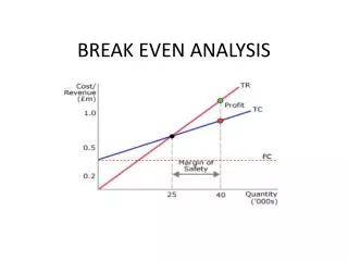
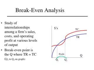
Break-Even Analysis. Study of interrelationships among a firm’s sales, costs, and operating profit at various levels of output Break-even point is the Q where TR = TC ( Q 1 to Q 2 on graph). $’s. TC. TR. Profit. Q. Q 1. Q 2. Linear Break-Even Analysis.

E N D
Break-Even Analysis Study of interrelationships among a firm’s sales, costs, and operating profit at various levels of output Break-even point is the Q where TR = TC (Q1 to Q2 on graph) $’s TC TR Profit Q Q1 Q2
Linear Break-Even Analysis • Over small enough range of output levels TR and TC may be linear, assuming • Constant selling price (MR) • Constant marginal cost (MC) • Firm produces only one product • No time lags between investment and resulting revenue stream
Graphic Solution Method TR • Draw a line through origin with a slope of P (product price) to represent TR function • Draw a line that intersects vertical axis at level of fixed cost and has a slope of MC • Intersection of TC and TR is break-even point $’s TC MC 1 unit Q FC P Q 1 unit Q Break-even point
Algebraic Solution • Equate total revenue and total cost functions and solve for Q TR = P x Q TC = FC + (VC x Q) TR = TC P x QB = FC + VC x QB (P x QB) – (VC x QB) = FC QB (P – VC) = FC QB = FC/(P – VC), or in terms of total dollar sales, PQ = (FxP)/(P-VC) = ((FxP)/P)/((P-VC)/P) = F/((P/P) – (VC/P)) = F/(1-VC/P)
Related Concepts • Profit contribution = P – VC • The amount per unit of sale contributed to fixed costs and profit • Target volume = (FC + Profit)/(P – VC) • Output at which a targeted total profit would be achieved
Example 1 – how many Christmas trees need to be sold • Wholesale price per tree is $8.00 • Fixed cost is $30,000 • Variable cost per tree is $5.00 • Solution Q(break-even) = F/(P – VC) = $30,000/($8 - $5) = $30,000/$3 = 10,000 trees
Example 2 – two production methods to accomplish same task • Method I : TC1 = FC1 + VC1 x Q • Method II : TC2 = FC2 + VC2 x Q • At break-even point: FC1 + (VC1 x Q) = FC2 + (VC2 x Q) (VC1 x Q) – (VC2 x Q) = FC2 – FC1 Q x (VC1 – VC2) = FC2 – FC1 Q = (FC2 – FC1)/(VC1 – VC2)
Example 2 continued: bowsaw or chainsaw to cut Christmas trees • Bowsaw • Fixed cost is $5.00 • Variable cost is $0.40 per • Chainsaw • Fixed cost is $305 • Variable cost is $0.10 per tree • Solution Q(break-even) = ($305 - $5)/($0.40 - $0.10) = 300/.30 = 1,000 trees
Fixed costs per acre: Land . . . . . . . $300 Site prep . . . . 100 Annual . . . . 60 Set-up . . . . . 5 Total . . . . 465 Variable costs per 100 seedlings Seedlings . . . . $ 5 Planting . . . . 20 Total . . . . 25 Example 3: Continued TC = 465 + 25 x (# trees per A/100)
Example 3: Continued • See Excel spreadsheet