Chapter 12 The Normal Probability Model

1. Chapter 12The Normal Probability Model

2. 12.1 Normal Random Variable • Black Monday (October, 1987) prompted • investors to consider insurance against • another “accident” in the stock market. How • much should an investor expect to pay for • this insurance? • Insurance costs call for a random variable that can represent a continuum of values (not counts)

3. 12.1 Normal Random Variable • Prices for One-Carat Diamonds

4. 12.1 Normal Random Variable • Percentage Change in Stock Market

5. 12.1 Normal Random Variable • X-ray Measurements of Bone Density

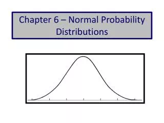
6. 12.1 Normal Random Variable • With the exception of Black Monday, the histogram of market changes is bell-shaped • Histograms of diamond prices and bone density measurements are bell-shaped • All three involve a continuous range of values; all three can be modeled using normal random variables

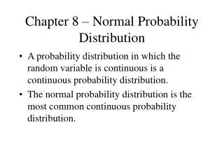
7. 12.1 Normal Random Variable • Definition • A continuous random variable whose • probability distribution defines a standard • bell-shaped curve.

8. 12.1 Normal Random Variable • Central Limit Theorem • The probability distribution of a sum of • independent random variables of comparable • variance tends to a normal distribution as the • number of summed random variables • increases.

9. 12.1 Normal Random Variable • Central Limit Theorem Illustrated

10. 12.1 Normal Random Variable • Central Limit Theorem • Explains why bell-shaped distributions are so common • Observed data are often the accumulation of many small factors (e.g., the value of the stock market depends on many investors)

11. 12.1 Normal Random Variable • Normal Probability Distribution • Defined by the parameters µ and σ2 • The mean µ locates the center • The variance σ2 controls the spread

12. 12.1 Normal Random Variable • Standard Normal Distribution (µ = 0; σ2 = 1)

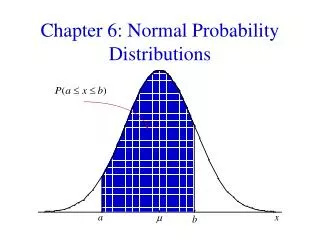
13. 12.1 Normal Random Variable • Normal Probability Distribution • A normal random variable is continuous and can assume any value in an interval • Probability of an interval is area under the distribution over that interval (note: total area under the probability distribution is 1)

14. 12.1 Normal Random Variable • Probabilities are Areas Under the Curve

15. 12.1 Normal Random Variable • Normal Distributions with Different µ’s

16. 12.1 Normal Random Variable • Normal Distributions with Different σ2’s

17. 12.2 The Normal Model • Definition • A model in which a normal random variable is • used to describe an observable random • process with µ set to the mean of the data • and σ set to s.

18. 12.2 The Normal Model • Normal Model for Diamond Prices • Set µ = $4,066 and σ = $738.

19. 12.2 The Normal Model • Normal Model for Stock Market Changes • Set µ = 0.94% and σ = 4.32%.

20. 12.2 The Normal Model • Normal Model for Bone Density Scores • Set µ = -1.53 and σ = 1.3.

21. 12.2 The Normal Model • Standardizing to Find Normal Probabilities • Start by converting x into a z-score

22. 12.2 The Normal Model • Standardizing Example: Diamond Prices • Normal with µ = $4,066 and σ = $738 • Want P(X > $5,000)

23. 12.2 The Normal Model • The Empirical Rule, Revisited

24. 4M Example 12.1: SATS AND NORMALITY • Motivation • Math SAT scores are normally distributed • with a mean of 500 and standard deviation of • 100. What is the probability of a company • hiring someone with a math SAT score of • 600 or more?

25. 4M Example 12.1: SATS AND NORMALITY • Method – Use the Normal Model

26. 4M Example 12.1: SATS AND NORMALITY • Mechanics • A math SAT score of 600 is equivalent z = 1. • Using the empirical rule, we find that 15.85% • of test takers score 600 or better.

27. 4M Example 12.1: SATS AND NORMALITY • Message • About one-sixth of those who take the math • SAT score 600 or above. Although not that • common, a company can expect to find • candidates who meet this requirement.

28. 12.2 The Normal Model • Using Normal Tables 27 of 45

29. 12.2 The Normal Model • Example: What is P(-0.5 ≤ Z ≤ 1)? • 0.8413 – 0.3085 = 0.5328

30. 12.3 Percentiles • Example: • Suppose a packaging system fills boxes such • that the weights are normally distributed with • a µ = 16.3 oz. and σ = 0.2 oz. The package • label states the weight as 16 oz. To what • weight should the mean of the process be • adjusted so that the chance of an • underweight box is only 0.005?

31. 12.3 Percentiles • Quantile of the Standard Normal • The pth quantile of the standard normal • probability distribution is that value of z such • that P(Z ≤ z ) = p. • Example: Find z such that P(Z ≤ z ) = 0.005. • z = -2.578

32. 12.3 Percentiles • Quantile of the Standard Normal • Find new mean weight (µ) for process

33. 4M Example 12.2: VALUE AT RISK • Motivation • Suppose the $1 million portfolio of an • investor is expected to average 10% growth • over the next year with a standard deviation • of 30%. What is the VaR (value at risk) using • the worst 5%?

34. 4M Example 12.2: VALUE AT RISK • Method • The random variable is percentage change • next year in the portfolio. Model it using the • normal, specifically N(10, 302).

35. 4M Example 12.2: VALUE AT RISK • Mechanics • From the normal table, we find z = -1.645 for • P(Z ≤ z) = 0.05

36. 4M Example 12.2: VALUE AT RISK • Mechanics • This works out to a change of -39.3% • µ - 1.645σ = 10 – 1.645(30) = -39.3%

37. 4M Example 12.2: VALUE AT RISK • Message • The annual value at risk for this portfolio is • $393,000 at 5% (eliminating the worst 5% of • the situations).

38. 12.4 Departures from Normality • Multimodality. More than one mode suggesting data come from distinct groups. • Skewness. Lack of symmetry. • Outliers. Unusual extreme values.

39. 12.4 Departures from Normality • Normal Quantile Plot • Diagnostic scatterplot used to determine the appropriateness of a normal model • If data track the diagonal line, the data are normally distributed

40. 12.4 Departures from Normality • Normal Quantile Plot • Normal Distributions on Both Axes

41. 12.4 Departures from Normality • Normal Quantile Plot • Distribution on y-axis Not Normal

42. 12.4 Departures from Normality • Normal Quantile Plot (Diamond Prices) • All points are within dashed curves, normality indicated.

43. 12.4 Departures from Normality • Normal Quantile Plot (Diamonds of Varying Quality) • Points outside the dashed curves, normality not indicated.

44. 12.4 Departures from Normality • Skewness • Measures lack of symmetry. K3 = 0 for • normal data.

45. 12.4 Departures from Normality • Kurtosis • Measures the prevalence of outliers. K4 = 0 • for normal data.

46. 12.4 Departures from Normality • Prices for Diamonds of Varying Quality

47. Best Practices • Recognize that models approximate what will happen. • Inspect the histogram and normal quantile plot before using a normal model. • Use z–scores when working with normal distributions.

48. Best Practices (Continued) • Estimate normal probabilities using a sketch and the Empirical Rule. • Be careful not to confuse the notation for the standard deviation and variance.

49. Pitfalls • Do not use the normal model without checking the distribution of data. • Do not think that a normal quantile plot can prove that the data are normally distributed. • Do not confuse standardizing with normality.