Analyzing Normal Distribution: Steel Rod Lengths & Worker Ratios
220 likes | 286 Vues
Explore examples of applying the normal distribution to steel rod lengths and worker ratios, along with assessing data normality using probability plots. Understand probability calculations and statistical tests in detail.

Analyzing Normal Distribution: Steel Rod Lengths & Worker Ratios
E N D
Presentation Transcript
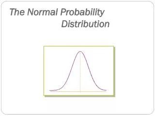
Chapter 7The Normal Probability Distribution 7.3 Applications of the Normal Distribution
EXAMPLE Finding the Area Under a Normal Curve It is known that the length of a certain steel rod is normally distributed with a mean of 100 cm and a standard deviation of 0.45 cm.* What is the probability that a randomly selected steel rod has a length less than 99.2 cm? *Based upon information obtained from Stefan Wilk.
EXAMPLE Finding the Area Under a Normal Curve It is known that the length of a certain steel rod is normally distributed with a mean of 100 cm and a standard deviation of 0.45 cm. What is the probability that a randomly selected steel rod has a length between 99.8 and 100.3 cm?
EXAMPLE Finding the Area Under a Normal Curve It is known that the length of a certain steel rod is normally distributed with a mean of 100 cm and a standard deviation of 0.45 cm. Suppose the manufacturer must discard all rods less than 99.1 cm or longer than 100.9 cm. What proportion of rods must be discarded?
EXAMPLE Finding the Area Under a Normal Curve It is known that the length of a certain steel rod is normally distributed with a mean of 100 cm and a standard deviation of 0.45 cm. Find the length corresponding to the 35th percentile.
EXAMPLE Finding the Area Under a Normal Curve It is known that the length of a certain steel rod is normally distributed with a mean of 100 cm and a standard deviation of 0.45 cm. Suppose the manufacturer wants to accept 90% of all rods manufactured. Determine the length of rods that make up the middle 90% of all steel rods manufactured.
Chapter 7The Normal Probability Distribution 7.4 Normal Probability Plots
Suppose that we obtain a simple random sample from a population whose distribution is unknown. Many of the statistical tests that we perform on small data sets (sample size less than 30) require that the population from which the sample is drawn be normally distributed. Up to this point, we have said that a random variable X is normally distributed, or at least approximately normal, provided the histogram of the data is symmetric and bell-shaped. This method works well for large data sets, but the shape of a histogram drawn from a small sample of observations does not always accurately represent the shape of the population. For this reason, we need additional methods for assessing the normality of a random variable X when we are looking at sample data.
A normal probability plot plots observed data versus normal scores. A normal score is the expected Z-score of the data value if the distribution of the random variable is normal. The expected Z-score of an observed value will depend upon the number of observations in the data set.
The idea behind finding the expected Z-score is that if the data comes from a population that is normally distributed, we should be able to predict the area left of each of the data values. The value of firepresents the expected area left of the ith data value assuming the data comes from a population that is normally distributed. For example, f1 is the expected area left of the smallest data value, f2 is the expected area left of the second smallest data value, and so on.
If sample data is taken from a population that is normally distributed, a normal probability plot of the actual values versus the expected Z-scores will be approximately linear.
We will be content in reading normal probability plots constructed using the statistical software package, Minitab. In Minitab, if the points plotted lie within the bounds provided in the graph, then we have reason to believe that the sample data comes from a population that is normally distributed.
EXAMPLE Interpreting a Normal Probability Plot The following data represent the time between eruptions (in seconds) for a random sample of 15 eruptions at the Old Faithful Geyser in California. Is there reason to believe the time between eruptions is normally distributed?
The random variable “time between eruptions” is likely not normal.
EXAMPLE Assessing Normality Suppose that seventeen randomly selected workers at a detergent factory were tested for exposure to a Bacillus subtillis enzyme by measuring the ratio of forced expiratory volume (FEV) to vital capacity (VC). NOTE: FEV is the maximum volume of air a person can exhale in one second; VC is the maximum volume of air that a person can exhale after taking a deep breath. Is it reasonable to conclude that the FEV to VC (FEV/VC) ratio is normally distributed? Shore, N.S.; Greene R.; and Kazemi, H. “Lung Dysfunction in Workers Exposed to Bacillus subtillis Enzyme,” Environmental Research, 4 (1971), pp. 512 - 519.