Normal distribution and probability

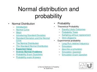
Normal Distribution Introduction Normal Curve Mean Introducing Standard Deviation Standard Deviation and the Normal curve The Normal Distribution The Standard Normal Distribution Expected Value Inverse Normal Problems Probability Exam Questions Probability exam Answers Probability Theoretical Probability Equally Likely Outcomes Probability Trees Sampling without replacement Venn diagrams Experimental probability Long-Run relative frequency Simulation describe a simulation Simulation Question Simulation Exam Question Normal distribution and probability L2 Normal Distribution & Probability M. Guttormson

Introduction L2 Normal Distribution & Probability M. Guttormson

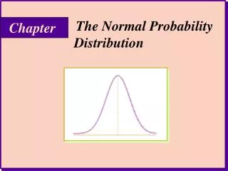
The Normal Curve • Many sets of data collected in nature, industry, business and other situations fit what is called a normal distribution. • This means: • If the frequency of each piece of data were graphed, the curve would fit a symmetrical bell shape. • Most measurements are near the middle • The further away from the middle value (mean), the less frequent the occurrence. • The general shape looks like this L2 Normal Distribution & Probability M. Guttormson

The Normal Curve L2 Normal Distribution & Probability M. Guttormson

Mean The mean is just the average of the numbers. It is easy to calculate: Just add up all the numbers, then divide by how many numbers there are. L2 Normal Distribution & Probability M. Guttormson

Introducing Standard Deviation The Standard Deviation (σ) is a measure of how spread out numbers are. You and your friends have just measured the heights of your dogs (in millimeters): The heights (at the shoulders) are: 600mm, 470mm, 170mm, 430mm and 300mm. Let’s find out the Mean and the Standard Deviation. L2 Normal Distribution & Probability M. Guttormson

Introducing Standard Deviation Answer: so the average height is 394 mm. Let's plot this on the chart: L2 Normal Distribution & Probability M. Guttormson

Introducing Standard Deviation Calculate the Standard Deviation using your calculators. Now we can show which heights are within one Standard Deviation (147mm) of the Mean: So, using the Standard Deviation we have a "standard" way of knowing what is normal, and what is extra large or extra small. Rottweillers are tall dogs. And Dachsunds are a bit short . L2 Normal Distribution & Probability M. Guttormson

Standard Deviation and the Normal Curve One standard deviation away from the mean in either direction on the horizontal axis (the red area on the graph) accounts for somewhere around 68 percent of the people in this group. “Likely/probable” Two standard deviations away from the mean (the red and green areas) account for roughly 95 percent of the people. “Very likely/very probable” Three standard deviations (the red, green and blue areas) account for about 99 percent of the people. “Almost certain” The total area under the curve adds to 1 (or 100%) L2 Normal Distribution & Probability M. Guttormson

The Normal Distribution L2 Normal Distribution & Probability M. Guttormson

The Standard Normal Distribution L2 Normal Distribution & Probability M. Guttormson

The Standard Normal Distribution Notation For the same question, calculate the percentage of cars travelling more than 97km/h? What is the probability that X is greater than 97km/h It is the probability that Z is greater than 0.2 This is equal to 1 – probability that Z is greater than 0.2 This is equal to 1 – 0.5793 Which is 42.07% L2 Normal Distribution & Probability M. Guttormson

Expected Value L2 Normal Distribution & Probability M. Guttormson

Inverse Normal Problems L2 Normal Distribution & Probability M. Guttormson

Equally Likely Outcomes L2 Normal Distribution & Probability M. Guttormson

0.1 0.04 Returned Kauri 0.4 Not Returned 0.36 0.9 0.05 Returned 0.03 Rimu 0.6 0.57 Not Returned 0.95 Probability Trees L2 Normal Distribution & Probability M. Guttormson

Probability Trees L2 Normal Distribution & Probability M. Guttormson

1/2 2/7 Blue Blue Red 2/7 1/2 2/3 Blue 2/7 Red 3/7 1/7 Red 1/3 Sampling Without Replacement 4/7 L2 Normal Distribution & Probability M. Guttormson

Venn Diagrams Union (one or the other or both) Intersection (both only) L2 Normal Distribution & Probability M. Guttormson

Venn Diagrams Complimentary Events P(A) is the probability inside the circle. P(A’) is the probability outside the circle. P(A) + P(A’)=1 Example: Probability that it rains tomorrow is 0.4. The probability that it does not rain tomorrow is 0.6 Mutually Exclusive Events Intersecting Events L2 Normal Distribution & Probability M. Guttormson

Long-run relative frequency L2 Normal Distribution & Probability M. Guttormson

Simulation L2 Normal Distribution & Probability M. Guttormson

How to describe a simulation Tool: Definition of the probability tool Statement of how the tool models the situation (Assign) “Generate random numbers using the random number key on a calculator and truncate. 12ran#+1=” “Designate numbers to colours of tee-shirts in the appropriate proportions. 1, 2 = blue 3, 4, 5 = red 6 = green 7, 8 = purple 9, 10 = yellow 11, 12 = black Trial: Definition of a trial Definition of a successful outcome of the trial “One trial would involve generating random numbers until there are seven outcomes representing each day of the week. Days need to be labelled Monday, Tuesday, Wednesday, Thursday, Friday, Saturday, and Sunday.” A successful trial would be if 3 or more of the same colour shirt appears in one trial (one week). L2 Normal Distribution & Probability M. Guttormson

How to describe a simulation • Results: Statement of how the results will be tabulated giving an example of a successful outcome and an unsuccessful outcome. • Statement of how many trials should be carried out. • “ A tick in the results column will indicate when 3 of the 7 random numbers generated represent the same colour tee-shirt. Repeat a minimum of 20 times.” • Calculation: Statement of how the calculation needed for the conclusion will be done: • Long run relative frequency = Number of successful results • Number of trials • Mean = Sum of trial results • Number of trials • The probabilities will be calculated using: Number of successful results • 20 L2 Normal Distribution & Probability M. Guttormson

Simulation Question L2 Normal Distribution & Probability M. Guttormson

Simulation Exam Question “T-shirts” L2 Normal Distribution & Probability M. Guttormson

Simulation Exam Question “Fair Cop” L2 Normal Distribution & Probability M. Guttormson

Probability exam Questions • QUESTION ONE • Andrew collected a large sample of chest measurements from students of his year level. • He found the chest measurements to be approximately normally distributed with a mean chest measurement of 86cm and a standard deviation of 3.5cm. • (a) Calculate the probability that a randomly selected student from Andrew’s year level • (i) would have a chest measurement between 86cm and 90cm • (ii) would have a chest measurement less than 87.5cm • (b) Andrew’s class has 34 students in it. How many of these students would you expect to have chest measurements of more than 89cm? L2 Normal Distribution & Probability M. Guttormson

Probability exam Questions L2 Normal Distribution & Probability M. Guttormson

Probability exam answers L2 Normal Distribution & Probability M. Guttormson

Normal distribution and probability