The Normal Probability Distribution
200 likes | 426 Vues
The Normal Probability Distribution. Some Basic Ideas. Review relative frequency histogram. Values of a variable, say test scores. 1/10 2/10 4/10 2/10 1/10. 60 70 80 90. In this example 10 people took a test. The height of each

The Normal Probability Distribution
E N D
Presentation Transcript
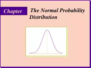
The Normal Probability Distribution Some Basic Ideas
Review relative frequency histogram Values of a variable, say test scores 1/10 2/10 4/10 2/10 1/10 60 70 80 90 In this example 10 people took a test. The height of each bar is the relative frequency or percentage of those in that range of scores. What % of people had test scores between 70 and 80? 40% What % of people had scores less than 70? 30% If you add up all the fractions what do you get? 1
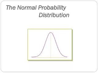
The Normal Distributions - Basic idea • The normal distribution is a tool we use to try to convey the same information as we get from a relative frequency histogram. • The normal distribution has been used a lot in statistics and we will use it later, so we will look at some details about it. • But, first let’s look at circles - yes I mean circles!
circles and density • Imagine you are at the intersection by Dairy Queen in Wayne. Now imagine a large circle is placed on the earth such that the center of the circle is at the intersection plus enough houses have been included so 1,000,000 people live in the circle. • New York City has a similar intersection and circle, except the circle is smaller (WHY?).
circles and density • You travel a shorter distance from the center to get an equal density of people in New York. • The smaller circle in a sense has a smaller standard deviation(actually it has a smaller radius) - the distance is less spread out. • One thing similar about the two circles is that you can divide them both up into quarters. Let’s do this on the next screen with two circles
circles and density A a 25% of the area is in A on the large circle and 25% of the area of the small circle is in part a. How can they both be 25%? It is 25 % of its own total. There are as many different normal distributions as there are circles. BUT, normal distributions are divided up, not into quarters, but in another way.
The Normal Distributions - normal dist. and density • Normal distributions can roughly be drawn by modifying a circle. flip this part out to left flip this part out to right like this
The Normal Distributions - normal dist. and density • Let’s label parts of the normal distributions. This point on the number line is directly below the inflection point. It turns out that the point on the number line is one standard deviation away from the center. This point is where the bottom part of the circle flipped. Let’s call it the inflection point. There is one on the other side as well. number line for the variable- like test score This is the center of the distribution. It really is the mean value we call mu
On the previous screen we see a graph of a normal distribution. Let’s consider an example to highlight some points. Say a company has developed a new tire for cars. In testing the tire it has been determined that the mean tire mileage is 36,500 miles and the standard deviation is 5000 miles. Along the horizontal axis we measure tire mileage. The normal distribution rises above the axis. Note the highest point of the curve occurs above the mean - in our tire example we would be at 36,500. On the curve we have two inflection points, and these occur 1 standard deviation away from the mean. So, mileages 31,500 and 41,500 are 1 standard deviation for the mean and the inflection points occur above them.
The Normal Distributions - notation • In general, now, we will talk about a variable having a normal distribution. We will say variable X is normally distributed with mean mu and standard deviation sigma. • More simply, we say X is N(mu,sigma). • Don’t let the N(---) part fool you, it means N(mean value listed first, then standard deviation value listed).
The Normal Distributions - example with graphical thinking • Say we have a variable X is N(3, 1) Why is this dot, and the one across, above #’s 2 and 4? X is measured on the line 4 2 3 Use the dots as your guide to draw the normal dist. 3 is the mean
The Normal Distributions - another example with graphical thinking • Say we have a variable X is N(3, 2) Why is this dot, and the one across, above #’s 1 and 5? X is measured on the line 4 5 1 2 3 Use the dots as your guide to draw the normal dist. 3 is the mean
The Normal Distributions - compare the two examples • here is what the two examples look like, one on top of the other X is N(3, 1) X is N(3, 2) 4 5 1 2 3
The Normal Distributions - compare the two examples • Note on the previous screen how the X is N(3, 2) had its inflection points wider than on the X is N(3, 1). • Remember how we labeled the quarters of the different circles A and a. We said there was 25% of the circle in both A and a, but based on its own total. • Normal dist.’s have a similar rule. 68% of the area under the curve is between the two inflection points. There is more.
The Normal Distributions - 68-95-99.7 rule • On any normal distribution the inflection points will be 1 standard deviation on either side of the mean. 68% of the area under the curve will be within this one standard dev. • By moving out 2 standard deviations on either side of the mean you have about 95% of the area under the curve. • By moving out 3 stand. dev.’s you have 99.7 % of the area under the curve.
The Normal Distributions - 68-95-99.7 rule • What is the meaning of the phrase, “1 standard dev. on either side of the mean?” • The answer is best seen by an example. X is (10, 2.5) means X is normal with mean 10 and standard deviation 2.5. Thus 7.5 is 1 stand. dev. on the low side of the mean and 12.5 is 1 stand. dev. on the high side of the mean. Thus being anywhere from 7.5 to 12.5 is within 1 standard deviation of the mean.
Note about normal distribution: 1. There are many normal distributions, each characterized by a mean value and a standard deviation. 2. The high point of the curve is above the mean and for a normal distribution the mean = median = mode. 3. Depending on the variable, the mean can be negative, zero, or positive. 4. The normal curve is symmetric. This means each side is a mirror image of itself. 5. Larger standard deviations result in a flatter, wider distribution. 6. Probabilities for the variable are found from areas under the curve - the 65, 95, 99.7 rule is an example of this.
26,500 31,500 36,500 41,500 46,500 miles -2 -1 0 1 2 z The concept of a z score is used with the normal distribution. z = ( a value minus the mean)/standard deviation. So the value 26,500 has a z = (26,500 - 36,500)/5000 = -2. This means 26,500 is 2 standard deviations below the mean. You can check the other values.