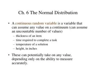
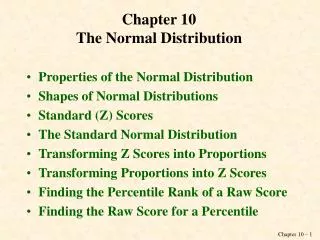
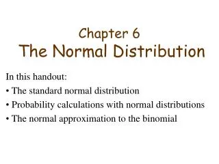
Chapter 6 The Normal Distribution
Chapter 6 The Normal Distribution. In this handout: Probability model for a continuous random variable Normal distribution. The idea of a continuous probability distribution draws from the relative frequency histogram for a large number of measurements (recall chapter 2).

Chapter 6 The Normal Distribution
E N D
Presentation Transcript
Chapter 6The Normal Distribution In this handout: Probability model for a continuous random variable Normal distribution
The idea of a continuous probability distribution draws from the relative frequency histogram for a large number of measurements (recall chapter 2). • Group data in class intervals, compute the relative frequencies of the intervals, and build a histogram (figure (a)). • The total area under the histogram is 1. • For two boundary points a and b of a class, the relative frequency of measurements in interval [a,b] is the area above this interval in the histogram. • With increasing number of observations, refine the histogram by having more class intervals with smaller widths (fig. (b)). • By proceeding in this manner, the jumps between consecutive rectangles tend to dampen out, and the top of the histogram approximates the shape of a smooth curve, as illustrated in figure (c). • This curve is called probability density curve.
Boxes on Page 223Probability density function; continuous random sample
For important distributions, areas have been extensively tabulated. • In most tables, the entire area to the left of each point is tabulated. • To obtain the probabilities of other intervals, we must apply the following rules: P[a < X < b] = (Area to left of b) – (Area to left of a)
Figure 6.2 (p. 225)Different shapes of probability density curves. (a) Symmetry and deviations from symmetry; (b) different peakedness.
Figure 6.3 (p. 225)Mean as the balance point and median as the point of equal division of the probability mass.
Figure 6.4 (p. 226)Quartiles of two continuous distributions.
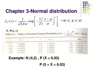
Statisticians often find it convenient to convert random variables to a dimensionless scale. E.g., if a random variable X has mean 400 and standard deviation 60, then the standardized variable is Z = (X - 400)/60
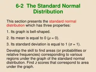
Normal distribution A bell-shaped distribution has been found to provide a reasonable approximation in many situations. The normal distribution with a mean of μ and a standard deviation of σ is denoted by N(μ, σ) . The curve never reaches 0 for any value of x, but because the tail areas outside (μ-3σ, μ+3σ) are very small, we usually terminate the graph at these points.
Figure 6.6 (p. 230)Two normal distributions with different means but the same standard deviation.
Figure 6.7 (p. 230)Decreasing increases the maximum height and the concentration of probability about .