Ch. 6 The Normal Distribution
Ch. 6 The Normal Distribution. A continuous random variable is a variable that can assume any value on a continuum (can assume an uncountable number of values) thickness of an item time required to complete a task temperature of a solution height, in inches

Ch. 6 The Normal Distribution
E N D
Presentation Transcript
Ch. 6 The Normal Distribution • A continuous random variable is a variable that can assume any value on a continuum (can assume an uncountable number of values) • thickness of an item • time required to complete a task • temperature of a solution • height, in inches • These can potentially take on any value, depending only on the ability to measure accurately.
The polygon of the distribution become a smooth curve called Probability Density Function (this is equivalent to Probability Distribution for discrete random variable) f(X) ) ≤ ≤ P ( a X b = ) < < P ( a X b X a b (Note that the probability of any individual value is zero)
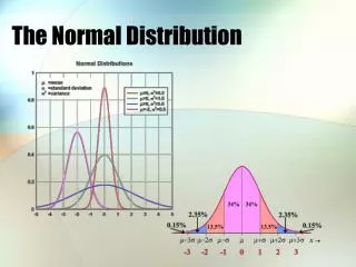
The Normal Distribution • Bell Shaped • Perfectly Symmetrical • Mean, Median and Mode are Equal • Location on the value axis is determined by the mean, μ Spread is determined by the standard deviation, σ • The random variable has an infinite theoretical range: + to f(X) σ + μ Mean = Median = Mode
What can we say about the distribution of values around the mean? There are some general rules: • Probability is measured by the area under the curve • The total area under the curve is 1.0, and the curve is symmetric, so half is above the mean, half is below • The height of the curve at a certain value below the mean is equal to the height of the curve at the same value above the mean • The area between: μ ± 1σ encloses about 68% of X’s μ ± 2σ covers about 95% of X’s μ ± 3σ covers about 99.7% of X’s
The Normal Distribution Density Function: • The formula for the normal probability density function is: (the curve is generated by): Where e = the mathematical constant approximated by 2.71828 π = the mathematical constant approximated by 3.14159 μ = the population mean σ = the population standard deviation X = any value of the continuous variable Note: f (X) is the same concept as P(X).
By varying the parameters μ and σ, we obtain different normal distributions. That is to say that any particular combination of μ and σ, will produce a different normal distribution. This means that we have to deal with numerous distribution tables. Changingμ shifts the distribution left or right. Changing σ increases or decreases the spread.
Standard Normal Distribution • Any normal distribution (with any mean and standard deviation combination) can be transformed into the standardized normal distribution (Z). • To do so, we need to transform all X units (values) into Z units (values) • Then the resulting standard normal distribution has a mean=zero and a standard deviation =1 • X-Values above the mean of X will have positive Z-value and X-values below the mean of will have negative Z-values • The transformation equation is:
EXAMPLE: • A sample of 19 apartment’s electricity bill in December is distributed normally with mean of $65 and std. dev. Of $9. Z- values for X = $83is: Z= (83-65)/9=18/9=2. That is to say that X=83 is 2 standard deviation above the mean or $65. Note that the distributions are the same, only the scale has changed. X (μ = 65, σ =9) 47 56 65 74 83 Z (μ = 0, σ =1) -2 -1 0 1 2
Applications: Use of Standard Normal Distribution Table, Pages 737-738 • What is the probability that a randomly selected bill is between $56 and $74?
What is the value of the lower 10% of the bills? (finding X value for a known probability)
What is the value of the highest 10% of the bills? (finding X value for a known probability)
What is the range of the values that contain the middle 95% of the bills?
Assessing Normality • Not all continuous random variables are normally distributed • It is important to evaluate how well the data set is approximated by a normal distribution • Construct charts or graphs • For small- or moderate-sized data sets, do stem-and-leaf display and box-and-whisker plot look symmetric? • For large data sets, does the histogram or polygon appear bell-shaped? • Compute descriptive summary measures • Do the mean, median and mode have similar values? • Is the interquartile range approximately 1.33 σ? • Is the range approximately 6 σ? • Observe the distribution of the data set within certain std. Dev. • Evaluate normal probability plot • Is the normal probability plot approximately linear with positive slope? Page 209


