Download
1 / 35
350 likes | 474 Vues
Regional Needs and Instrumentation for CO 2 Observations. Britton Stephens, NCAR ASP Colloquium, June 11, 2007. Outline. Background Regional Needs CO 2 Measurement Techniques AIRCOA Example Sources of potential bias Regional Applications of in situ CO 2 Observations.

E N D
Regional Needs and Instrumentation for CO2 Observations Britton Stephens, NCAR ASP Colloquium, June 11, 2007
Outline • Background • Regional Needs • CO2 Measurement Techniques • AIRCOA Example • Sources of potential bias • Regional Applications of in situ CO2 Observations
Carbon cycle science as a field began with the careful observational work of Dave Keeling Keeling, C.D., Rewards and penalties of monitoring the earth, Annu. Rev. Energy Environ., 23, 25-82, 1998.
Background CO2 measurements define global trends and loosely constrain continental-scale fluxes TransCom 3 Study Fluxes 2 1 0 -1 -2 60 30 0 -30 -60 Pg C / yr Billion $ Expected from fossil fuel emissions
TEMPERATURE (C) (IPCC, 2001) (NRCS/USDA, 1997) Regional scale is critical for linking to underlying processes (NRCS/USDA, 1997) CHLOROPHYLL (SeaWIFS, 2002)
Continental mixed-layer CO2 is highly variable Rocky RACCOON CO2 Concentrations April 2007 NWR Mean Diurnal Cycle and Hourly Variability June 2006 TURC/NDVI Biosphere Takahashi Ocean EDGAR Fossil Fuel [U. Karstens and M. Heimann, 2001]
Using high frequency data makes signals bigger, but the annual-mean signals are still very small: To measure 0.2 GtCyr-1 source/sink to +/- 25% need to measure regional annual mean gradients to 0.1-0.2 ppm Flux footprint, in ppm(GtCyr-1)-1, for a 106 km2 chaparral region in the U.S. Southwest (Gloor et al., 1999).
Important Definitions 2 instruments over time in the field 1 instrument over several seconds 1 instrument over time in the lab 1 instrument over time in the field [ Recommendations of the 13th WMO/IAEA Meeting of Experts on Carbon Dioxide Concentration and Related Tracers Measurement Techniques, http://www.wmo.int/pages/prog/arep/gaw/documents/gaw168.pdf ]
Absolute Measurement Techniques: Manometric and Gravimetric NOAA/CMDL Manometer: Reproducibility of 0.06 ppm (C. Zhao et al., 1997) Keeling manometer has run since ’50s
Relative Measurement Techniques: Non-dispersive Infrared (NDIR) Spectroscopy • Broadband IR radiation filtered for 4.26 um • Cooled emitter and detector • Pulsed emitter or chopper wheel • 1 or 2 detection cells (from www.tsi.com) Advantages: Robust, precise, affordable Disadvantages: Non-linear; sensitivity to pressure, temperature, and optical conditions; pressure broadening
LiCor, Inc. CO2 Analyzer CMDL Flask Analysis System
Cavity Ringdown Spectroscopy (CRDS) Advantages: Precise, extremely stable Disadvantages: Somewhat more expensive, relatively new
Relative measurements require calibration gases tied to a common scale NOAA/CMDL scheme for propagation of WMO CO2 scale: For NDIR, generally 4 points needed for 0.1 ppm comparability Recalibration needed ~ every 3 years due to drift
Autonomous, Inexpensive, Robust CO2 Analyzer (AIRCOA) • 0.1 ppm precision and 0.1 ppm comparability on a 2.5 min. measurement • $10K in parts and operates autonomously for months at a time
Automated web-based output http://raccoon.ucar.edu
Field Surveillance Tanks Mean offsets (and standard deviations) of these measurements from the laboratory-assigned values were: ‑0.08 (+/- 0.11), -0.07 (+/- 0.11), and -0.01 (+/- 0.07) ppm at the three sites. NOAA GMD Flask Comparisons The NOAA flasks have a mean offset and standard deviation relative to our measurements of 0.01 ppm +/- 0.18 ppm.
Map of existing North American continuous well-calibrated CO2 measurements. Colors denote measuring group, with Rocky RACCOON sites in Red. Courtesy of S. Richardson (http://ring2.psu.edu). Map showing existing Rocky RACCOON sites (red), proposed new sites (purple), and potential future sites (gray). Continuous, well-calibrated CO2 measurements across North America Towers over 650 feet AGL in U.S.
Point-to-Point Flux Estimates NWR – SPL = -2.1 ppm CO2 HYSPLIT back-trajectory calculation for the afternoon of June 17, 2006 (6 PM LT), over topography (GoogleEarth Pro). The EDAS 40 km meteorology used for this simulation predicts that air which passed near SPL at 2 PM LT reached NWR at 6 PM LT. Using the observed CO2 difference and the model transit time of 260 minutes, the model boundary-layer heights of 2000 m at SPL and 1878 m at NWR, an average atmospheric pressure of 60 kPa over this column, and a simple Lagrangian box model, we obtain a first-order flux estimate of -0.31 gC m‑2 hr‑1. This value compares reasonably well with the 1999-2003 average flux for late afternoon in June from the Niwot Ridge AmeriFlux Site of -0.2 gC m‑2 hr‑1 (S. Burns, personal communication).
Monthly-mean Boundary-layer Budgeting Monthly mean filtered CO2 concentrations at the 4 Rocky RACCOON sites and differences from marine boundary layer concentrations interpolated to the same latitude. With estimates of boundary-layer depth can estimate fluxes, following on: Bakwin, P.S., K.J. Davis, C. Yi, S.C. Wofsy, J.W. Munger, L. Haszpra, and Z. Barcza (2004), Regional carbon dioxide fluxes from mixing ratio data, Tellus, 56B, 301-311. Helliker, B.R. et al. (2004), Estimates of net CO2 flux by application of equilibrium boundary layer concepts to CO2 and water vapor measurements from a tall tower (DOI 10.1029/2004JD004532). Journal of Geophysical Research, 109, D20106. Styles, J.M., P.S Bakwin, K. Davis, B.E. Law (2007), A simple daytime atmospheric boundary layer budget validated with tall tower CO2 concentration and flux measurements, in press.
Inversion / Data-assimilation on Finer Scales http://www.esrl.noaa.gov/gmd/ccgg/carbontracker/index.html
Influence-function Optimization of Simple Ecosystem Models Figures from: Matross, D. M., A. Andrews. M. Pathmathevan, C. Gerbig, J.C. Lin, S.C. Wofsy, B.C. Daube, E.W. Gottlieb, V.Y. Chow, J.T. Lee, C. Zhao, P.S. Bakwin, J.W. Munger, and D.Y. Hollinger (2006). Estimating regional carbon exchange in New England and Quebec by combining atmospheric, ground-based and satellite data, Tellus, 58B, 344-358. Also stay tuned for: Richardson, S.J., N.L. Miles, K.J. Davis, M. Uliasz, A.S. Denning, A.R. Desai, and B.B. Stephens (2007), Demonstration of a high-precision, high-accuracy CO2 concentration measurement network for regional atmospheric inversions, J. Atmos. Oceanic Technol., to be submitted.
Regional Scale Lagrangian Experiment “Moving columns” wind direction Day 1: late PM Day 2: early AM Day 2: late PM Mixed layer top [ Figure courtesy of John Lin ]
North Dakota Observations CO2 CO upstream downstream [ Figure courtesy of John Lin ]
Airborne Carbon in the Mountains Experiment (ACME-07) Flight June 7, 2007 Figure produced by S. Aulenbach, A. Desai, and D. Moore
Dry Mole Fraction of CO2 For ± 0.1 ppm consistency, need to stabilize to ± 300 ppm H2O (or dry to dewpoint of -25 ºC)
Intra- and Inter-laboratory agreement still not better than 0.2 ppm
Automated Flask Sampling (from www.cmdl.noaa.gov/ccgg)
Light Aircraft Profile Carr, Colorado, USA (from www.cmdl.noaa.gov/ccgg)
13CO2/12CO2 and O2/N2 Ratios [R. Keeling, SIO] Independent constraints on the land-ocean partitioning of CO2 fluxes [NOAA/CMDL]
Satellite CO2 Measurements Advantages: Dramatic increase in CO2 data, consistent global coverage, total column abundances, comparable to other datasets Disadvantages: Potential for biases due to aerosols, clouds, land surface type, viewing angle, or sun angle, expensive Thermal Infrared Emission: Available, but primarily mid to upper troposphere Reflected Near Infrared:
800 m 360 m 120 m Representativeness COBRA-2000 Daytime Profiles Total representativity error of mixed layer averaged CO2 mixing ratios (combined observational error and representativity error) plotted against the horizontal dimension of the region. Vertical bars indicate the 5-95% range. [Gerbig et al., submitted to JGR] S