Introduction to Statistical Process Control
Introduction to Statistical Process Control. Module 4. History of Statistical Process Control. Quality Control in Industry Shewhart and Bell Telephones Deming & Japan after WWII Use in Health Care & Public Health. The Run Chart. The Count. Cups of Coffee. Day. The Mean.

Introduction to Statistical Process Control
E N D
Presentation Transcript
History of Statistical Process Control • Quality Control in Industry • Shewhart and Bell Telephones • Deming & Japan after WWII • Use in Health Care & Public Health
The Count Cups of Coffee Day
The Mean The mean of 4, 7, 8 , and 2 is equal to: 4+7+8+2 4
The Median-Odd Numbers • = the middle value in an ordered series of numbers. • To take the median of 1, 7, 3, 10, 19, 4, 8 • Order these numbers: 1,3,4,7,8,10,19 • The median is zth number up the series where z=(k+1)/2 and k=number of numbers. • What is the median in this case?
The Median-Even k • Order the numbers, i.e., 1,7,10,14,15, 17. • Find the middle values, i.e., 10 and 14. • Take the average between these two values. • What is the median?
The Proportion You have these 10 values representing 10 people: 0,0,0,1,0,1,0,0,1,0. Zero means person did not get sick. One means person did get sick. What is the mean of these 10 values? (0+0+0+1+0+1+0+0+1+0)/10 = .333 Proportion= n/N, where n=number of people who got sick and N=total number of people. n=numerator, N=denominator.
What is a population? • A group of people? • A group of people over time? • Hospital visits? • Motor vehicle crashes? • Ambulance Calls? • Vehicle-Miles? • X-Rays Read? • Other?
Populations take onDistributions In simple statistical process control, we deal with 4 distributions.
From central tendency to variation. The Normal Distribution
How do we describe variation about the red line in the normal curve? • In other words, how fat is that distribution? • How about the average difference between each observation and the mean? • Oops, can’t add those differences, some are positive and some are negative. • How about adding up the absolute values of those differences? • Bad statistical properties. • How about the average squared difference? • Now we are talking!
Population Variance N ∑ 1 Population Variance = (xi - µ)2 N i=1 The average squared deviation!
Population Standard Deviation N Population Standard Deviation = ∑ √ 1 (xi - µ)2 N i=1 The square root of the average squared deviation!
How do I estimate the standard deviation of the means of repeated samples? • Estimate the standard deviation of the population with your sample using the sample standard deviation. • Estimate the standard deviation of the mean of repeated samples by calculating the standard error.
Sample Standard Deviation N ∑ √ 1 S = (xi - x)2 N-1 i=1 How is this different from the Population Standard Deviation?
Standard Error s SE = √ n How is this different from the Sample Standard Deviation?
Z-Score for Distribution of Sample Means x - μ Z = SE X = mean observed in your sample μ = is the population mean you believe in. Z = number of standard errors x is away from μ, You can convert any group of numbers to z-scores.
If we kept dancing for hundreds of times Here is the distribution of our sample means (standardized)
Wait a minute! • When you do a survey, you only have one sample, not hundreds of repeated samples. • How confident can you be that the mean of your one sample represents the mean of the population? • If you think reality is a normal distribution with mean y and standard deviation s, how likely is your observed mean of x?
Welcome to • Confidence Intervals • P-Values • Let’s focus on p-values for now.
Here is the mean we observed (1.96 ≈ 2) Here is our distribution of sample means—WE BELIEVE What is the probability of observing a mean at least as far away as zero (on either side) as 1.96 standard errors? 2.72? Area under curve is probability and it adds up to one. .025 .025
Remember the p-value question? • If you think reality is a normal distribution with mean y and standard deviation s, how likely is your observed mean of x?
Let’s ask it again. • We have systolic blood pressure measurements on a sample of 50 patients for each of 25 months. For each of those months, we a mean blood pressure and a sample standard deviation. • “You think reality for each month should be a normal distribution with a mean blood pressure that equals the average of the 25 mean blood pressures. • You also think that for each month, this normal distribution should have a standard error based on the average sample standard deviation across the 25 months. • How likely is your observed mean in month 4 of 220 if the average mean across the 25 months was 120? • How many standard errors is 220 away from 120? What is the probability of being at least that many standard errors away from 120?
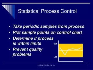
Welcome to the Shewart Control Chart 1 2 3 4 5 6 7 . . . 25 120
Anatomy of the control chart: From Amin, 2001 Indian Health Service, DHHS