Download

1 / 41
410 likes | 443 Vues
Panther Creek Lidar Sets and Growth Estimation. Jim Flewelling. Western Mensurationist meeting June 18-20, 2017 Vancouver, BC. Support through Agenda 2020 Technology Alliance (FS Agreement 11-JV-11261989-036). Outline. Panther Creek Overview Yield estimates over time.

E N D
Panther Creek Lidar Sets and Growth Estimation Jim Flewelling Western Mensurationist meeting June 18-20, 2017 Vancouver, BC Support through Agenda 2020 Technology Alliance (FS Agreement 11-JV-11261989-036).
Outline Panther Creek Overview Yield estimates over time. Estimating change in yield Top height
2300 ha watershed near Portland, Oregon Douglas fir natural and planted stands. Also hemlock, cedar, grand fir, red alder, bigleaf maple. 100 m – 700 m elevation. Extensive data.
Cooperative Agreement Statement on Cooperative Watershed Research in the Panther Creek Watershed “All data developed as part of the cooperative research in Panther Creek is considered public information and is available to anyone upon request.” Supplemental Data Sharing Agreement. “All parties recognize that some of the material may be of a preliminary nature and may contain errors.”
Tree Measurement Plots 84 plots, 0.08 ha, stem mapped Six subjectively selected Sampling design for some Others near soil pits. Measurements: 2009, late in growing season; 2012, late summer or fall; 2016, before growing season. Six plots: just two measurements.
Tree Measurement Plots Down Woody Debris, 2011 Hemispherical photos, 2011
Other Data TLS (RSGAL, Monika Moskal and students), 2011 Center scan only: 19 plots Center plus 3 edge scans: 27 plots Soils: EPA (Mark Johnson) Weather stations: OSU, Doug Maquire
Intermediate Results Clipped lidar plots (90 m by 90 m). DEMs and Lidar metrics by plot. Colocation offsets. Yield metrics by plot. Interpolations and extrapolations. Delineated ITCs Steams (RSGAL, Jeff Richardson) Stream nodes and Stahler Stream orderWhen are results stable enough to be usefully shared?
Intermediate result: Tree data Tree sizes projected to end of growing season. Tree sizes extrapolated back to reference year 2007. Probabilistic mortality for trees in 2007 and 2008. Annual interpolations: tree and/or per hectare.
Intermediate result: Co-location • Panther Creek: • Target coordinates assigned for plot centers. • GPS used to install plots at those targets. • Cadastral survey with expected 0.5 m accuracy. • Want to tie stem mapped tree data to lidar returns. • Find center offset (x, y) and angular offset. • Subjective decisions or subjective algorithm
Co-location Methodology • ALS data is the reference data set and is assumed to be correct. • Start with the cadastral determinations of plot centers. • Find the (x,y) offset to plot center and the angular adjustment needed to adjust the stem-mapped plot. • Prefer an automated approach.
Co-location example with largest adjustment Plot 200110 70 m clip.
Delineated Crowns Field plot should be centered within the 40 m box.
Delineated Crowns Red circle: 16.2 m radius about cadastral plot center. Crown centroids also shown.
Tree Map TREE MAP Circle: 16.2 m radius. Square: 40 m side. 9DF50 implies Tag = 9 Sp = DF Ht = 50 m X : Dead L: Leaning
Trees and Multi-temporal tops. Example: 16M51~6.9 ID: 16 Height(2012)= 51 m Free radius no higher returns up to 6.9 m
TREES and Multi-temporal Tops after co-locations. Shift in Trees: X +1.6 m Y + 3.6 m Angle + 2 deg. mse (dist) = 0.60 Mse (ht) = 0.40
Tree-Top Matching Compare (Xmod, Ymod) with (TopX, TOPY), and H-tree with H-top
Per hectare yield predictions • Leaf-on data sets: 5 years, separate and combined. • Leaf-off data sets: 5 years separate and combined. • Dependents: • BA basal area (m2/ha) • HL lorey height (m) • VOL whole stem volumes (cvts, m3/ha( • LN_VOL natural log of VOL
Regressions, LN_VOL, Leaf-on 2007 is an outlier?
Regressions, LN_VOL, Leaf-off Leaf-off : better MSEs
Regressions, LN_VOL, Leaf-on, Evaluate on combined data 2015 is the outlier, Why?
Regressions, Cross-evaluations, Leaf-off LN_VOL
Per-hectare yield regressions • Mean-square errors are large. • Differences between data sets can not be ignored. • Species inference should help.
General Option for Growth • Y = Predicted Y2 – Predicted Y1 • With separate regressions, Y1 and Y2 • With a common regression. • With a common regression plus offset. • Y = f(X) • Y = f(X1 ,X2 )
One growth result for volume • Predict Volume 2010 to 2015. • Lidar data 2010/07 and 2015/06. • Model:V = exp(b0 + b1 Elev2 +b2 PC2) - exp(a0 + a1 Elev1 +a2 PC1) • ResultsV has mean = 70.8 m3. StDev 48.9RMSE = 45.7 (6.5% of variance explained)
Top height • Top height often defined as the expectation of a protocol similar to:average height of n largest diameter trees on a plot of a specified size (Rennolls, 1978, Garcia, 1998). • Similar concept invoked here:On lidar plot, identify 25 possible tree tops.Calculate mean of the nine tallest.
Lidar top height increment 201007 to 201506 Tallest nine crown tops. Some outliers due to changes in top selection
Tree height errors are small • If we identify and follow highest lidar points on individual trees, errors in implied growth are usually less than one year’s growth. • Extreme example follows plot 109804 , tree 13 Douglas fir with 165 cm diameter.
Infer site index, averaging increments of dominant trees? • Most site curves can be displayed as:family of h versus h. • Mean h and h for dominant trees in a stand can be found from successive lidar flights. • Assign site index to stands or parts of stands?
Synergy for Multitemporal Lidar • Two acquisitions (with field data). • Estimate height growth and site index. • Use site index as an independent variable in estimating yield.
Thank you Special thanks to George McFadden, David Marshall, Steve Reutebuch Bob McGaughey, Connie Harrington, Van Kane, Qi Chen,, Russ Faux, Monika Moskal, and all Panther Creek participants.