OBS 1: Microwave Limb Sounding
460 likes | 904 Vues
OBS 1: Microwave Limb Sounding. COST 723 UTLS Summerschool Cargese, Corsica, Oct. 3-15, 2005 Stefan A. Buehler Institute of Environmental Physics University of Bremen www.sat.uni-bremen.de. Overview. Basics of limb sounding instruments Basics of the measurement

OBS 1: Microwave Limb Sounding
E N D
Presentation Transcript
OBS 1: Microwave Limb Sounding COST 723 UTLS Summerschool Cargese, Corsica, Oct. 3-15, 2005 Stefan A. Buehler Institute of Environmental Physics University of Bremen www.sat.uni-bremen.de
Overview • Basics of limb sounding instruments • Basics of the measurement • Past, present, and future instruments • Summary
Overview • Basics of limb sounding instruments • Geometry • Antenna • Radiometry • Basics of the measurement • Past, present, and future instruments • Summary
Geometry ho: Platform altitude θ: Scan angle ht: Tangent altitude typically: RE = 6000 km ho = 600 km ht = 6-60 km • Measure thermal radiation from the atmosphere (passive!) • Good altitude resolution, because we can scan vertically
Small ∆θ↔ large ∆ht. Accurate Pointingnecessary. Narrow Field of Viewnecessary. (Figure: Oliver Lemke)
Antenna (Figure: Oliver Lemke) • Field of view diameter = “beam width”, even for passive instrument • Given by angle of half power of received (or transmitted) radiation • Diffraction theory:θHPBW~ Wavelength / Antenna size
Antenna Technology • θHPBW~ Wavelength / Antenna size • Needs large antenna, particularly for low frequencies • Scan angle small • Needs accurate scanning mechanism (or wobble the whole satellite) The Odin reflector mounted on the spacecraft body. (Source: PREMIER mission proposal)
The Radiometer Challenge • The absolute power of thermal radiation in the mm-wave spectral range is low.
(Kraus, J. D., Radio Astronomy, McGraw-Hill Book Company, 1966)
The Radiometer Challenge • The absolute power of thermal radiation in the mm-wave spectral range is low. (The peak of the Planck function is in the infrared.) • Need to amplify the signal by many orders of magnitude for detection. • No good amplifiers for frequencies above approximately 100 GHz (technology constantly moving) • State of the art: Heterodyne Receivers
A Typical Heterodyne Radiometer RF = Radio frequency LO = Local oscillator IF = Intermediate frequency (Figure: Oliver Lemke)
The Heterodyne Principle (Figure: Oliver Lemke) • Mixer generates signal with νIF = | νRF - νLO | • This can then be amplified and analyzed with a spectrometer • Intensity unit: Brightness temperature = The temperature a black body would need to generate the same intensity of radiation
The Radiometer Formula TNET = Noise equivalent temperature (noisiness of individual measurement) TSys = System noise temperature (characteristic noise of measurement system) ΔB = Frequency bandwidth Δt = Integration time
The Radiometer Challenge (2) • We cannot make ΔB and Δt as large as we want. (We want spectral resolution, and the satellite flies by fast.) • Need low noise receivers. • Mixer and first amplifier most critical, because their noise is amplified by subsequent stages. • Cool mixer to low operation temperature. Best: Superconducting (SIS) mixers at 4 K. • Cooled HEMT amplifiers.
Submillimeter-wave Sensor at –269 C SMILES Superconductive Device: Nb/AlOx/Nb 640 GHz SIS Mixer 0.4 mm 4 K 20 K 100 K 4 K Mechanical Cooler SIS: Superconductor-Insulator-Superconductor (Figures: SMILES Team)
Overview • Basics of limb sounding instruments • Basics of the measurement • Spectroscopy • Limb Spectra • Clouds • Past, present, and future instruments • Summary
Microwave Spectroscopy Absorption by a gas (Lambert-Beer’s Law):
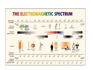
Absorption coefficient αdetermined by • Continua • Electronic transitions (1015 Hz, UV visible) • Vibrational transitions (1013 Hz, Infrared) • Rotational transitions (1011Hz, mm / sub-mm)
Limb Spectra O3 H2O (Emde et al., J. Geophys. Res., 109(D24), D24207, 2004)
Comparison to IR Limb Sounder • Annual global mean probability of limb transmittance >3%, as estimated from ECMWF fields of temperature, water vapour, water and ice clouds sampled globally one day in ten over a year (Kerridge et al., ESA UTLS study final report). • Clouds significant, but less critical than for IR
Overview • Basics of limb sounding instruments • Basics of the measurement • Past, present, and future instruments • UARS-MLS and MAS (past) • EOS-MLS and Odin (present) • SMILES and PREMIER (future) • Summary
The first two Microwave Limb Sounders O2 63 GHz H2O 183 GHz O3 184 GHz ClO 205 GHz MAS MLS ‘Millimeterwave Atmospheric Sounder’ ‘Microwave Limb Sounder’ On the Space ShuttleOn the UARS satellite Atlas 1, March 19921991-1998 Atlas 2, April 1993 Atlas 3, November 1994
A sample MAS H2O Measurement MAS Water Vapor Band MMC 20075, 27.3.1992, 16.59 GMT 59° N 021° W, Tangent altitude range: 6-54 km • Retrieval = Calculate trace gas profile from measured spectra • Requires radiative transfer model = forward model
UARS/MLS Highlights • Stratospheric ozone and chlorine chemistry research • Impact of volcano eruptions on the stratosphere (SO2 loading) • Tropical dynamics (‘tape recorder’ effect in the tropical lower stratosphere). • Publication overview at: http://mls.jpl.nasa.gov/joe/um_pubs.html
(Source: MLS Website. See also: Read et al., Geophys. Res. Lett. 20, 1299-1302, 1993.)
The Tropical LS Taperecorder Deviation from mean VMR [ppm] • Transit time from 100 to 46 hPa > 6 months • (Data created by H. Pumphrey. See also: Mote et al. J. Geophys. Res., vol. 101, 3989-4006 [1996])
EOS MLS • The next Generation of the Microwave Limb Sounder MLS • Launched July 15, 2004, on the Aura satellite (Figure: MLS Webpage)
EOS MLS Observed Species (WATERS, et al.: EOS MLS ON AURA, IEEE GRS submitted 2005)
Odin • Small satellite with just two limb sounders, one sub-mm, one UV-visible • The whole platform is moved, not just the antenna • Launched February 20, 2001 • Frequencies:118.25 - 119.25 GHz 486.10 - 503.90 GHz 541.00 - 580.40 GHz
JEM / SMILES • ‘Superconducting Sub-Millimeter Wave Limb Emission Sounder’ • Launch 2008 on the ‘Japanese Experimental Module’ (JEM) of the International Space Station • SIS mixer, cooled to < 4 Kelvin • Proof of concept for later instruments of this type • Very accurate ozone and chlorine species data • Measurements at 625 and 650 GHz
PREMIER • Combined IR and sub-mm limb imagers • Proposed to current ESA call, possible launch 2013 • Focus on chemistry climate interaction in the UTLS • Sub-mm measurements at 320-360 GHz • Array detectors • Main Products: O3, H2O, CO, N2O, HNO3, ClO, CH4, CFC11, CFC12, C2H6, SF6
Overview • Basics of limb sounding instruments • Basics of the measurement • Past, present, and future instruments • Summary
Summary (1) • Limb sounding is well suited for the measurement of trace gases in the stratosphere and upper troposphere. • Particularly good for chlorine species and humidity. (Also many other trace gases.) • Good altitude resolution (1–2 km). • Horizontal resolution is ≈ 100 km. • We look at emission linesof trace gases. • Emission means continuous measurement, day & night.
Summary (2) • Less affected by clouds than UV and IR techniques. • Cirrus clouds must be taken into account in the UT. • Past: UARS-MLS and MAS. • Present: EOS-MLS and Odin. • Future: SMILES? PREMIER? Third generation of MLS? • Technological challenges are low noise receivers with large bandwidth. Antenna size is also always a cost factor.