Binomial Probability Distribution
This overview explores the Binomial Probability Distribution (BPD), a key concept in probability theory. It relates to experiments with two possible outcomes, such as flipping a coin or determining whether a car starts. In a binomial experiment, we analyze the likelihood of success across multiple trials. We discuss critical aspects such as the counting rule, combinations, and the role of independent events. With practical examples and calculations, this guide simplifies the process of determining probabilities, empowering users to apply these principles effectively in various scenarios.

Binomial Probability Distribution
E N D
Presentation Transcript
Binomial Probability Distribution Here we study a special discrete PD (PD will stand for Probability Distribution) known as the Binomial PD
Examples When you flip a coin you will see face up either a heads or a tails. When you go to start your car by putting the key in the ignition switch and turning either the car will start or it will not start. When a customer goes into a store either a purchase will be made or a purchase will not be made. Note in each example only 2 possible outcomes can occur. We will call one outcome a success, s, and the other outcome a failure, f. Maybe the successes are heads, car starts, and a purchase is made in the examples, respectively.
Binomial experiment We can expand on each example on the previous slide by thinking about each example being repeated what we say is a general number n times. We will be specific about n in particular problems. Say we flip a coin 5 times. Say we think about cold winter days and we see how many days the car starts on the next 7 days. Say we wonder how many of the next 6 customers will make a purchase.
Counting Rule 1 If any one of b different mutually exclusive and collectively exhaustive events can occur on each of n trials, the number of possible outcomes is equal to bn (b raised to the nth power). Sometimes this will be written as b^n, where ^ means the next number should be treated as a power. In any binomial problem b = 2. If you flip a coin 5 times 2^5 = 32 different outcomes. If you start the car seven straight days 2^7 = 128 outcomes. If you observe the next 6 customers 2^6 = 64 outcomes.
The binomial random variable is the number of successes that occur in the n trials. The number of successes is either 0, 1, 2, 3, 4 up to the n trials. In the coin flipping example where we flip the coin 5 times and heads is a success we could have the outcome of the five flips as ssssf or sssfs or ssfss or sfffs or 32 total outcomes like this. Note here I show 3 ways of having 4 successes in the 5 flips.
Rule 5 Combinations – The formula for the number of combinations when taking x objects from n objects, irrespective of order is n!/[X!(n - X)!]. For example 4 from 5 has combinations 5! = (5)(4)(3)(2)(1) = (5) = 5 4!(5 - 4)!(4)(3)(2)(1) 1 So, n is the number of trials in the binomial context and x is the number of successes.
If we start the car 7 times the number of ways we can have 4 starts is 7!/[4!(7- 4)! = 7(6)(5)/3(2) = 35. Some of these include ssssfff, sssfsff, sssffsf. There are 35 of these types. Let’s play with starting the car a little more here. Let’s say on any one try the probability the car starts – a success – is .99. This means the probability of a failure is .01. If each day the car starting is an independent event from any other day then the probability of the car starting on the first 4 days and not the last 3 is .99(.99)(.99)(.99)(.01)(.01)(.01) = .0000009. The probability it starts on the first 3 days, then not on the next 3 and then it does on the last day is .99(.99)(.99)(.01)(.01)(.01) (.99)= .0000009. This is where my calculator stops, but the answer was rounded. So the probability the car starts on any 4 days is .0000009(35) = .0000315. In Microsoft Excel I get 3.36209E-05 = .000336209
So the probability the car starts on any 4 days is .0000009(35) = .0000315. In Microsoft Excel I get 3.36209E-05 = .000336209. What is going on here? I have no idea! Really though, since .0000009 can occur 35 different ways we just have .0000009(35).
On the next 2 slides I want to show you what Microsoft Excel can do for you when you have a binomial problem. On the next slide the column x has the number of successes in 7 trials. Then second column has the probability of the x in the row. For example, the probability of 4 successes in 7 trials is 3.36209E-05 = .000336209. The third column is the cumulative probability. This means in a given row take the probability of that x and add to it all the previous probabilities. You can think of this column then as the probability of an x amount or less than that amount. For example in the x = 4 row we have 3.39625E-05 = .0000339625. 2 screens from now I show what to type in Excel to get the results.
You may have noticed this is not a class in Excel and you should not use Excel here (but you can if you want – except on tests.) But I want to tell you this story so far because we will really use a table in the back of the book to get binomial probabilities. Starting on page 303 you see binomial probability tables. Small n is the number of trials, p is the probability of a success on 1 trial, and k is related to a specific value for x. Remember x is the number of successes on n trials. In fact, inside the table are the cumulative probabilities. For example, when n = 7, p = .99 and k = 6 the number .0679 is the probability of having 6 or fewer successes in 7 trials. The .0020 is the probability of having 5 or fewer successes in 7 trials. What is the probability of having exactly 6 successes in 7 trials? The answer is found by taking the number for 6 or fewer and subtracting the number for 5 or fewer to get .0679 - .0020 = .0659.
In the Excel file we saw that directly, but our table wants to economize on the use of ink and paper so we are shown minimum amounts of information and we can piece the rest together. Hey, when n =7 why is there no k = 7 row? The answer is because the number should always accumulate to 1.00. What is the probability of having 7 successes in 7 trials when p = .99? 1 - .0679 = .9321. Let’s see what a binomial process contains.
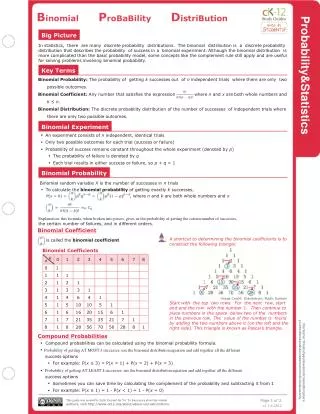
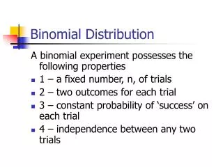
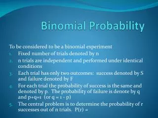
Properties of a Binomial process. 1) The are a fixed number of observations or trials, n. 2) Each observation is classified into one of two mutually exclusive and collectively exhaustive categories. One category will be labeled a success and the other a failure. 3) The probability of an observation being classified as a success, denoted by p, is constant (does not change) from observation to observation. q = (1 - p) is the probability of an observation being classified as NOT successful, or a failure, and does not change from observation to observation. 4) The observations are independent.
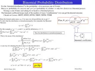
In general, the probability, written p(x), of a given x is found by the formula n! px(1-p)(n-x) remember something raised to 0 power = 1 x!(n-x)! And we will use the table to get these values.
The expected value for the binomial PD is = np(a simplification for the binomial case from what we saw previously for a discrete random variable), and the variance is Var(x) = σ2 = np(1-p) (also a simplification). The standard deviation is just the square root of the variance. Consider a binomial experiment with n = 10 and p = 0.1. a. using the table in the back of the book we have .3487 b. using table in the back of the book we have .9298 - .7361 = .1937 c. P(x≤2) is in the book as .9298 d. P(x≥1) = 1 – P(x≤0) = 1 - .3487 = .6513.
Example 6.4 starting on page 87. Note n = 10 and p = .2 a. From the table .1074 b. Take the 2 or fewer number and subtract the 1 or fewer number to get .6778 - .3758 = .3020


