Path Analysis
Path Analysis. Path Diagram. Single headed arrow runs from cause to effect Double headed bent arrow: correlation The model above assumes that all 5 variables are turned into z-scores (standardized) It can be represented by a set of standardized STRUCTURAL (regression) equations:

Path Analysis
E N D
Presentation Transcript
Path Diagram • Single headed arrow runs from cause to effect • Double headed bent arrow: correlation • The model above assumes that all 5 variables are turned into z-scores (standardized) • It can be represented by a set of standardized STRUCTURAL (regression) equations: • Occ=.281*1stOc+.394*Ed+.115*FaOc+e1 • 1stOc=.440*Ed+.224*FaOc+e2 • Ed=.279*FaOc+.310*FaEd+e3 • a. Exogeneous vs. Endogeneous Variables • Exogenous variables are never dependent variables: FaOcc, FaEd • Endogenous variables are dependent variables at least once: Occ, 1stOc, Ed • b. Dependent vs, Independent Variables • While the exogenous vs. endogenous distinction is with respect to the model as a whole, D vs. I variables are defined with respect to individual equations • c. Recursive vs. Non-Recursive Models • A recursive model is one where the flow of causation is one-way: you start from any variable and if you follow the one headed arrows, you cannot encounter the same variable twice
Structural Equations • EQ1: • PREMARSX=a+b1*RELITEN+b2*EDUC+e • EQ2: • ABSINGLE=a’+b1’*RELITEN+b2’EDUC+b3’*PREMARSX+e’ • Standardized Structural Equations • EQ1: • Zpremarsx=ppr*Zreliten+ppe*Zeduc+e1 • EQ2: • Zabsingle=par*Zreliten+pae*Zeduc+pap*Zpremarsx+e1 • pyx= the path (standardized regression) coefficient of X in a regression where X is one independent and Y is the dependent variable Observed Variables UnobservedVariables
Normal Equations • for each equation the number of normal equations is K where K= number of independent variables • rvariable1, variable2= rvariable2,variable1bivariate Pearson’s correlation coefficient measuring the linear relationship between x and y • EQ1: • 1) • rreliten,premarsx=ppr*rreliten,reliten+ppe*rreliten,educ+ rreliten,e1 as rreliten,reliten=1 and rreliten,e1=0 • rreliten,premarsx=ppr +ppe*rreliten,educ • 2) • reduc,premarsx=ppr*rreliten,educ +ppe • EQ2: • 3) • rreliten,absingle =par +pae*rreliten,educ + pap*r reliten,premarsx, • 4) • reduc,absingle =par* reduc, reliten +pae + pap*reduc, premarsx • 5) • rpremarsx,absingle=par* rpremarsx,reliten +pae*rpremarsx,educ+ pap • 5 normal equations, 5 path coefficients: 5 equations, 5 unknowns: JUST-IDENTIFIED model
Effects of Religion (RELITEN) on Support for Abortion for Single Women (ABSINGLE) • Take the normal equation which has the correlation of RELITEN and ABSINGLE on the right-hand side (Normal Equation #1) for EQ2). • rreliten,absingle =par +pae*rreliten,educ + pap*r reliten,premarsx, • Notice that • rreliten,premarsx=ppr +ppe*rreliten,educ (Normal Equation #1 for EQ1). • So • rreliten,absingle =par + pae*rreliten,educ+ pap*( ppr +ppe*rreliten,educ)= • rreliten,absingle =par + pae*rreliten,educ+ pap* ppr + pap*ppe*rreliten,educ • Total direct unanalyzed indirect unanalyzed • association= effect + effect through +effect through + effect through • education premarital sex education AND • premarital sex
Decomposing the relationship between intensity of religious beliefs and support for abortion for single women • Direct effect = -.074 • Indirect effect through Premarsx = -.291*.335= -.097485 • Unanalyzed effect due to Educ = -.019*.230= -.00437 • Unanalyzed effect due to Educ and Premarsx= -.019*.171*.335= -.001088415 • Total association = -.074 +-.097485 +-.00437 +-.001088415 = -.176943415 • Compare to rAbsingle,Reliten = -.177 e2 e1 Reliten -.074 -.291 .335 Absingle Premarsx -.019 .171 Educ .230
Effects of Education (EDUC) on Support for Abortion for Single Women (ABSINGLE) • Take the normal equation which has the correlation of RELITEN and ABSINGLE on the right-hand side (Normal Equation #2) for EQ2). • reduc,absingle =par* reduc, reliten +pae + pap*reduc, premarsx • Notice that • reduc,premarsx=ppr*rreliten,educ +ppe (Normal Equation #2 for EQ1) • So • reduc,absingle =par* reduc, reliten +pae + pap* (ppr*rreliten,educ +ppe)= • reduc,absingle =par* reduc, reliten +pae + pap* ppr*rreliten,educ + pap* ppe • Total unanalyzed direct unanalyzed indirect • association= effect through + effect + effect through + effect through • religion religion and premarital sex • premarital sex
Decomposing the relationship between education and support for abortion for single women • Direct effect = .230 • Indirect effect through Premarsx = .171*.335= .057285 • Unanalyzed effect due to Reliten = -.019*-.074 = .001406 • Unanalyzed effect due to Reliten and Premarsx= -.019*-.291*.335=.001852215 • Total association = .230+ .057285 + .001406 +.001852215= 0.290543215 • Compare to rAbsingle,Educ= .291 e2 e1 Reliten -.074 -.291 .335 Absingle Premarsx -.019 .171 Educ .230
Effects of support for pre-marital sex on Support for Abortion for Single Women • Take the normal equation which has the correlation of PREMARSX and ABSINGLE on the right-hand side (Normal Equation #3 for EQ2). • rpremarsx,absingle=par* rpremarsx,reliten +pae*rpremarsx,educ+ pap • Notice that • rreliten,premarsx =ppr +ppe*rreliten,educ (Normal Equation #1) for EQ1). • (keep in mind that rreliten,premarsx=rpremarsx, reliten) • and • reduc,premarsx=ppr*rreliten,educ +ppe (Normal Equation #2) for EQ1) • So • rpremarsx,absingle=par*( ppr +ppe*rreliten,educ )+pae*( ppr*rreliten,educ +ppe )+ pap= • rpremarsx,absingle =par* ppr + par* ppe*rreliten,educ +pae* ppr *rreliten,educ + pae *ppe + pap • Total association unanalyzed unanalyzed association direct • association= due to + effect through + effect through + due to + effect • common cause education and religion and common cause • religion religion education education
Decomposing the relationship between attitude towards pre-marital sex and support for abortion for single women • Direct effect = .335 • Spurious effect due to common cause Reliten = .-.291*-.074= .021534 • Spurious effect due to common cause Educ = .171*.230= .03933. • Unanalyzed effect due to correlation of common cause Reliten with Educ= -.291* -.019*.230= .00127167 • Unanalyzed effect due to correlation of common cause Educ with Reliten= .171*-.019*-.074= .00074727 • Total association = .335 + .021534+ .03933+ .00127167+ .00074727=.039788294 • Compare to rAbsingle,Premarsx= .398 e2 e1 Reliten -.074 -.291 .335 Absingle Premarsx -.019 .171 Educ .230
Rules of calculating the various effects of (X) on (Y) • a. Direct effect • path coefficient • b. Indirect effects • Start from the variable (Y) later in the causal chain to your right. Trace backwards (right to left) against arrows passing intervening variables until you get to variable (X) • Each combination of intervening variables is a separate indirect effect. • c. Spurious effects (due to common causes) • Start from variable (Y). Trace backwards to a variable (Z) that has a direct or indirect effect on both (X) and (Y). Move from (Z) to (X). • There are as many spurious effects of (X) on Y due to (Z) as many ways you can get from Y to (X) through (Z) following the rule above. • d. Correlated (unanalyzed) effects • If (X) is one of several exogenous variables find (Z) that is both exogenous and has a direct or indirect effect on Y. Start from variable (Y). Trace back to (Z). Make the last step through the double headed arrow to (X) • If (X) is an endogenous variable, find an exogenous variable (Z) that has a direct or indirect effect on (Y) and is correlated to another exogenous variable (W) that has a direct or indirect effect on (X). Start from variable (Y). Trace back to (Z). Travel through the double headed arrow to (W). Move from (W) to (X). • Comment: A Correlated (unanalyzed) effect is like an indirect effect or a spurious effect due to common causes, except it includes one (and only one) double headed arrow.
Rules of calculating the total association • 1. Find all paths • Sewall Wright's rules • No loops • Within one path you cannot go through the same variable twice. • No going forward then backward • Only common causes matter, common consequences (effects) don't. • Maximum of one curved arrow per path • 2. Calculate compound paths (indirect, spurious, correlated) by multiplying coefficients encountered on the way • 3. Add up all direct and compound effects
Identification of fully recursive models Rules of thumb (The actual rules of identification are bit more complicated but the following rules will work most of the time) • Just-Identified Models • As many coefficients as normal equations (a necessary but not sufficient condition) • With K variables this means k*(k-1)/2 single headed and double headed arrows • Just-identified models can be estimated in SPSS as separate regression equations. • Underidentified Models • More coefficients than normal equations • Underindentified models cannot be estimated • A model can be locally underidentified even when you have the same or more normal equations than coefficient to estimate. • Overidentified Models • Fewer coefficients than normal equations (a necessary but not sufficient condition) • Degrees of freedom: = #normal equations-#coefficients