PATH ANALYSIS
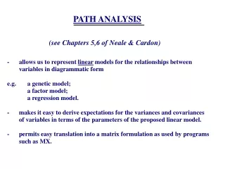
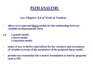
PATH ANALYSIS. (see Chapters 5,6 of Neale & Cardon). -. allows us to represent. linear. models for the relationships between. variables in diagrammatic form. e.g. a genetic model;. a factor model;. a regression model. -.

PATH ANALYSIS
E N D
Presentation Transcript
PATH ANALYSIS (see Chapters 5,6 of Neale & Cardon) - allows us to represent linear models for the relationships between variables in diagrammatic form e.g. a genetic model; a factor model; a regression model. - makes it easy to derive expectations for the variances and covariances of variables in terms of the parameters of the proposed linear model. - permits easy translation into a matrix formulation as used by programs such as MX.
ADDITIVE DOMINANCE GENETIC UNIQUE SHARED GENETIC e.g. EFFECT ENVIRONMENT ENVIRONMENT EFFECT E A C D 1 1 1 1 e a c d P PHENOTYPE P = eE + aA + cC + dD
Figure 1. A PATH MODEL FOR MZ TWIN PAIRS 1.0 1.0 (MZT) or 0.0 (MZA) 1.0 1 EXOGENOUS D D C C E A E A 1 1 1 1 1 1 1 T1 T2 T1 T2 T1 T1 T2 T2 VARIABLES e a c d e a c d ENDOGENOUS P P T1 T2 VARIABLES TWIN 1 TWIN 2
CONVENTIONS OF PATH ANALYSIS Squares or rectangles denote observed variables. Circles or ellipses denote latent (unmeasured) variables. Upper-case letters are used to denote variables. Lower-case letters (or numeric values) are used to denote covariances or path coefficients. Single-headed arrows or paths ( ) are used to represent hypothesized causal relationships between variables under a particular model -- where the variable at the tail of the arrow is hypothesized to have a direct causal influence on the variable at the head of the arrow (e.g., A P ). T1 T1
Double-headed arrows ( ) are used to represent a covariance between two variables, which may arise through common causes not represented in the model. Double-headed arrows ( ) may also be used to represent the variance of a variable. Double-headed arrows may be used for any variable which has one or more not single-headed arrows pointing to it -- these variables are called endogenous variables. Other variables are exogenous variables. Single-headed arrows may be drawn from exogenous to endogenous variables (A P) or from endogenous variables to other endogenous variables (P P ). 1 2
Omission of a two-headed arrow between two exogenous variables implies the assumption that the covariance of those variables is zero (e.g., no genotype-environment correlation). Omission of a direct path from an exogenous (or endogenous) variable to an endogenous variable implies that there is no direct causal effect of the former on the latter variable.
ASSUMPTIONS OF OUR SIMPLE PATH MODEL FOR MZ TWIN PAIRS : (i) linear additive effects -- no multiplicative (genotype x environment) interactions; (ii) E, A, C, D are mutually uncorrelated -- no genotype-environment covariance; (iii) path coefficients e, a, c, d are the same for first, second twins; (iv) no reciprocal sibling environmental influences; i.e., no direct paths P P 1 2
(Simplified rules assuming no ‘feedback loops’, i.e., no reciprocal causation - • reciprocal sibling environmental influences - etc.) • (1) Trace backwards, change direction at a 2-headed arrow, then trace • forwards. • implies that we can never trace through two 2-headed arrows in • the same chain. • (2) The expected covariance between two variables, or the expected • variance of a variable, is computed by multiplying together all the • coefficients in a chain, and then summing over all possible chains. TRACING RULES OF PATH ANALYSIS
e.g., for the MZ twin pair covariance we have: CONTRIBUTION a 1 a a2 c 1 c d 1 d CovMZ = a2 + c2 + d2 P1 AT1 AT2 P2 P1 CT1 CT2 P2 c2 P1 DT1 DT2 P2 d2
e.g., for the total phenotypic variance for MZ twins: CONTRIBUTION e 1 e e2 a 1 a c 1 c d 1 d VarMZ = e2 + a2 + c2 + d2 P1 ET1 ET1 P1 P1 AT1 AT1 P1 a2 P1 CT1 CT1 P1 c2 P1 DT1 DT1 P1 d2
PATH ANALYSIS: EXERCISES Exercise 1.Using Figure 1, what is the expected covariance between MZ twin pairs reared apart (MZAs)? Exercise 2. Using Figure 1, what is the expected variance of twins from MZ pairs reared apart?
Figure 2. DZ TWIN PAIRS/FULL SIBLINGS 0.25 1 (DZT/FST) or 0 (DZA/FSA) 0.5 (1+x) 1 1 1 1 1 1 1 1 D E A C E A C D d e h c e h c d P P TWIN 1 TWIN 2 x = 0 under random mating.
Exercise 3. Using Figure 2, and assuming random mating (x=0), what is the expected covariance between DZ twin pairs reared together? Exercise 4. Using Figure 2, what is the expected variance of DZ twins or full siblings reared together? Exercise 5. Using Figure 2, what is the expected covariance of DZ twins or full sibling pairs reared apart?
Figure 3. BIOLOGICAL PARENT - OFFSPRING 1 1 1 1 1 1 1 1 E C A D E C A D d a c e a e c d 0.5 0.5 0.5 0.5 P P MOTHER FATHER 1 0.5 R R 0.5 A 0.25 A 1 1 E C A D D A C E 1 1 1 1 1 1 e c h d d h c e P P CHILD 2 CHILD 1
Exercise 6. Using Figure 3, what is the expected covariance of parent and offspring? Exercise 7. Using Figure 3, what is the expected covariance of biological parent and adopted-away offspring? Exercise 8. What 10 assumptions are implied by Figure 3?
Figure 4. BIOLOGICAL UNCLE / AUNT - NEPHEW / NIECE 1 0.5 0.25 E C A D E C A D E C A D e c a d e c a d e c a d 0.5 P 0.5 FATHER P P AUNT/UNCLE MOTHER R 0.5 1 A E C A D e c a d P NEPHEW/NIECE
Exercise 9. Using Figure 4, what is the expected covariance between biological uncle and nephew?
Figure 5. OFFSPRING OF MZ TWIN PAIRS 1 1 1 1 1 1 1 1 1 1 1 E D C A E D C A A C D E A C D E 1 1 1 1 1 1 1 1 e d c a e d c a a c d e a c d e ½ ½ ½ ½ PSPOUSE1 PSPOUSE2 PTWIN1 PTWIN2 0.5 0.5 R R A A 1 1 1 E D A C E D A C 1 1 1 e d a c e d a c POFFSPRING (Twin 2) POFFSPRING (Twin 1)
Exercise 10. Using Figure 5, what is the expected covariance between MZ uncle/aunt and nephew/niece, i.e. between an MZ twin and the child of his or her cotwin? Exercise 11. What is the expected covariance between first cousins related through MZ twins (“MZ half sibs”)?
Figure 6. DIRECTION-OF-CAUSATION MODEL: MZ PAIRS 1 E C E C 1 1 1 1 e c e c CONDUCT PROBLEMS TWIN 1 CONDUCT PROBLEMS TWIN 2 i i 1 E A E A 1 1 1 1 e a e a ALCOHOL DEPENDENCE TWIN 1 ALCOHOL DEPENDENCE TWIN 2
Exercise 12. Using Figure 6, (1) What is the expected MZ covariance for (a) conduct problems; (b) alcohol dependence; (c) conduct problems in one twin and alcohol dependence in the cotwin? (2) Redraw Figure 6 so that the direction of causation is now ALCOHOL DEPENDENCE CONDUCT PROBLEMS What are the expected MZ covariances now for (a) conduct problems; (b) alcohol dependence; (c) conduct problems in one twin and alcohol dependence in the cotwin?
(3) What are the corresponding expected DZ covariances when (a) CONDUCT PROBLEMS ALCOHOL DEPENDENCE (b) ALCOHOL DEPENDENCE CONDUCT PROBLEMS
PART TWO: PATH ANALYSIS: FROM PATH DIAGRAMS TO MATRICES It is straightforward to convert from a path diagram to a matrix representation of a path model, and vice versa. Here we illustrate a computationally efficient approach - though other alternatives exist (see e.g. the MX manual). Consider first a model with no feedback loops --for example Figure 1 for MZ twin pairs reared together, where all endogenous variables are directly observable, and there are no paths from endogenous variables to other endogenous variables. Let X denote the covariance matrix for the exogenous variables. The i, j-th element of the matrix X (where i denotes R ow, and j denotes C olumn) will be equal to the covariance of the i-th, j-th exogenous variables. will be a matrix. X square
1.0 0.0 0.0 0.0 0.0 0.0 0.0 0.0 0.0 1.0 0.0 0.0 0.0 1.0 0.0 0.0 0.0 0.0 1.0 0.0 0.0 0.0 1.0 0.0 0.0 0.0 0.0 1.0 0.0 0.0 0.0 1.0 X = MZ 0.0 0.0 0.0 0.0 1.0 0.0 0.0 0.0 0.0 1.0 0.0 0.0 0.0 1.0 0.0 0.0 0.0 0.0 1.0 0.0 0.0 0.0 1.0 0.0 0.0 0.0 0.0 1.0 0.0 0.0 0.0 1.0
Let denote the matrix of paths from the exogenous variables to the endogenous W variables. The i, j-th element of the matrix will be equal to the path from the j-th W exogenous variable to the i-th endogenous variable. will be a matrix, rectangular W with number of rows equal to the number of endogenous variables, number of columns equal to the number of exogenous variables. e a c d 0 0 0 0 = W 0 0 0 0 e a c d
For this simplified case, with no paths from endogenous variables to other endogenous variables, and all endogenous variables directly observable, we can derive the expected covariance matrix as a product of matrices, SMZ = WXMZ W
e a c d 0 a c d = WX 0 a c d e a c d e a c d 0 a c d e 0 = WXW 0 a c d e a c d a 0 c 0 d 0 0 e 0 a 0 c 0 d 2 2 2 2 2 2 2 e + a + c + d a + c + d = S MZ 2 2 2 2 2 2 2 a + c + d e + a + c + d
Exercise 13. Using Figure 2, write down the elements of the covariance matrix of the exogenous variables for DZ pairs, XDZ. SDZ = WXDZ W Derive
Figure 7 represents a more complicated model, with paths from endogenous variables to other endogenous variables -- in this example, representing the reciprocal environmental influences of the twins upon each other (or perhaps a rater contrast effect, if twin data are ratings by the same parent).
Figure 7. MODEL WITH RECIPROCAL SIBLING EFFECTS 0.25 1 (MZ) or (DZ/FS) 1 (MZT/DZT/FST) or 0 (MZA/DZA/FSA) 0.5 1 (MZ) or (DZ/FS) D E A C E A C D d e a c e a c d 0 (MZA/DZA/FSA) or i (MZT/DZT/FST) P P TWIN 1 TWIN 2 0 (MZA/DZA/FSA) or i (MZT/DZT/FST) i - reciprocal sibling interaction effect
It may be shown , again assuming that all endogenous (see Neale and Cardon, C6) variables are directly observable, that SMZ = ZWXMZ W Z -1 where Z = (I - Y) SDZ = ZWXDZ W Z and Here is the identity matrix, and denotes the inverse. -1 I
Exercise 14. What are the expected covariance matrices for MZ and DZ twin pairs reared together, and for MZ and DZ twin pairs reared apart, under the model of Figure 7?
Exercise 15. Redraw Figure 6 for the case of reciprocal causation, i.e. a path i from ALCOHOL DEPENDENCE to CONDUCT PROBLEMS, in addition to the path i from CONDUCT PROBLEMS to ALCOHOL DEPENDENCE. What is the expected 4x4 covariance matrix for MZ pairs for this case?