HWRF PHYSICS
HWRF PHYSICS. Hurricane WRF Tutorial NCWCP College Park, MD Jan 14 2014. Young C. Kwon EMC/NCEP/NOAA. Contents. Overview Land surface model Surface layer physics (air-sea interaction) Planetary Boundary Layer Convective parameterization Micro-physics Radiation


HWRF PHYSICS
E N D
Presentation Transcript
HWRF PHYSICS Hurricane WRF Tutorial NCWCP College Park, MD Jan 14 2014 Young C. Kwon EMC/NCEP/NOAA
Contents Overview Land surface model Surface layer physics (air-sea interaction) Planetary Boundary Layer Convective parameterization Micro-physics Radiation Physics upgrade plan for FY2014
Overview At the initial operational implementation, HWRF physics suite was closely following as GFDL hurricane model physics. Some physics are from GFS (PBL, convection), some are originated from NCEP mesoscale model (Micro-Physics) and others are from GFDL (radiation, surface physics, Land surface), and modify to tropical environment. Many aspects of physics have been upgraded, and the 2013 HWRF physics will be covered in this presentation. The proposed 2014 physics upgrades will also introduced briefly.
HWRF model Physics suite *: plan to upgrade at 2014
Thermodynamic equation vertical advec. + adiabatic heating H. diffusion diabatic heating Time tendency horizontal advection where, Diabatic heating: phase change of water – convection, microphysics Radiative absorption/emission – radiation Subgrid vertical mixing – PBL, convection Surface fluxes – air-sea interaction, land surface
physics Radiative cooling/warming micro-physical processes subgrid scale mixing subgrid scale convection Dynamics Horizontal/vertical advections, horizontal diffusion
Land surface modelGFDL hurricane model slab ∂T*/∂t = (-σT*4 - Shfx - Levp + (S+F ))/ρscsd)
Verification of HWRF Skin temperature over CONUS (compare to GFS analysis)
Air-sea interactions Hurricane intensity is proportional to sqrt(Ch/Cd) over ocean – Emanuel(1995) Upper level outflow Hurricane Energy gain from sea surface (sensible and latent heat) Ch Low level inflow Energy loss by surface friction Cd OCEAN
Ck: Surface exchange coefficient for moisture & heat Cd: Surface exchange coefficient for momentum Ch before modification ChX103 CdX103 10m Wind speed (m/s) 10m Wind speed (m/s) Km: Eddy diffusivity for momentum Km: Eddy diffusivity for momentum Cd and Ch profile in the current HWRF model (gray dots) Modified GFS Scheme Original GFS Scheme Same Observations
CBLAST data (2007) HEXOS data(1996, Decosmo et al) Original HWRF/GFDL model
PBL scheme: Parameterize subgrid-scale vertical turbulence mixing of momentum, heat and moisture in the boundary layer. There are two main categories of PBL schemes: local vs non-local mixing scheme. Local mixing scheme: vertical mixing is proportional to the local gradient., e.g. Mellor-Yamada-Janjic scheme, Blackadar scheme Non-local mixing scheme: vertical mixing is not only proportional to local gradient but also counter-gradient mixing due to large scale eddy, e.g., GFS scheme, YSU scheme. HWRF model uses GFS PBL scheme, which is non-local mixing scheme. GFS PBL has shown to good performance outside of hurricane regions while PBL height in hurricane area is too deep and too strong mixing compare to observational data. Recent PBL scheme upgrades address this issue significantly.
Procedures in the operational HWRF PBL scheme 1. First guess PBL height PBL 2. Update using the first guess PBLh 3. Enhance PBLh using updated 4. Momentum diffusivity (Km) is calculated under PBLh z (1 - z/h) p 5. Moist diffusivity (Kt) is calculated using Prandtl number
Introduce to match Km to obs z (1 - z/h) p Cd Ch Km Km Gopalakrishnan et al (2012)
Reduction of momentum diffusivity led to shallower PBL height and inflow depth Gopalakrishnan et al (2012)
Variable Critical Richardson number (Vickers & Mahrt, 2003) Motivation: The GFS PBL scheme used in HWRF model has been known to produce too diffusive boundary layer in hurricane condition. Thanks to HRD’s effort to improve the hurricane PBL in HWRF model, the diffusivity and PBL height of HWRF model greatly improved based on composite dropsonde observations (e.g., Gopalakrishnan et al. 2013, JAS; Zhang et al. 2013, TCRR) PBL z (1 - z/h) p However, outside of hurricanes, the GFS PBL behaves quite well and some underestimation of PBL height is reported (Jongil Han, personal communication). Therefore, it may worth trying to revise the current PBL scheme to work well in both inside and outside of hurricane area seamlessly.
Critical Richardson number function of Ro (Vickers and Mahrt, 2003) Vickers and Mahrt(2003) Critical Richardson number is not a constant but varies with case by case. Hurricane cases Ric = 0.16(10−7 )−0.18 The magnitude of Ric modifies the depth of PBL and diffusivity, so the Ric varying with conditions would fit both hurricane condition and environments.
PBL height difference (new PBL scheme with varRic – PBL scheme in 2012 HWRF with constant Ric=0.25) Hurricane Katia (20110829018+96hr) PBL height over the ocean and hurricane area becomes shallower while that over land area becomes deeper Both configurations have set to 0.5
Convective parameterization: When grid resolution of a numerical model is too coarse to resolve individual convection, there are need to parameterize the impact of convection to grid scale. Convection does stabilized the atmospheric column by vertical transportation of heat, moisture and momentum. There are two main categories in convective parameterization scheme. One is an adjustment scheme and the other is a mass flux scheme. HWRF model uses Simplified Arakawa Shubert (SAS) which is one of the mass flux scheme. Grid point value
SAS deep convection scheme CTOP 0.1A DL A hs hs h LFC hc 120-180mb SL Environmental moist static energy Updated SAS scheme Courtesy from Jongil Han (EMC)
Mean sea level pressure (hPa) analysis 27 Sep 2000, 12 UTC Spurious? No momentum mixing 132-h forecasts with various amounts of momentum mixing Too intense ? momentum mixing Han and Pan 2006
Microphysics scheme: While convective parameterization scheme is parameterizing subgrid/unresolvable moist processes, microphysics scheme predict the behavior of hydrometeo species explicitly. Hence, microphysics scheme are called explicit moisture scheme, grid scale precipitation scheme or large scale precipitation scheme . There are bulk microphysics schemes (which are widely used in NWP models) and bin microphysics scheme. HWRF uses Ferrier microphysics schemewhich is a single moment bulk scheme.
Cloud MicrophysicsTropical Ferrier scheme • mp_physics=85 • Very similar to current NAM general Ferrier scheme Differences in RH condensation onset, number concentration, etc • Designed for efficiency • Advection only of total condensate (CWM) and vapor • Diagnostic cloud water, rain, & ice (cloud ice, snow/graupel) from storage arrays (F_*) • Assumes fractions of water & ice within the column are fixed during advection • Supercooled liquid water & ice melt • Variable density for precipitation ice • (snow/graupel/sleet) – “rime factor” (F_rime)
Qt=Qi+Qr+Qc (CWM = ice mixing ratio+rain mixing ratio + cloud water mixing ratio) Qi = Fice * Qt Ql = (1-Fice) * Qt Qr= Ql * Frain = (1-Fice) * Frain * Qt Qc = (1-Frain)* Ql =(1-Fice) * (1-Frain) * Qt F_rime = F_rime should be always bigger than 1. Based on F_rime value, ice species are defined like, snow/sleet/grauple
T < 0oC WaterVapor T > 0oC IEVP CND Cloud Ice PrecipIce(Snow/Graupel/Sleet) DEP REVP CloudWater IACW ICND IACWR RAUT RACW IACR Rain IMLT Sfc Snow/Graupel/Sleet Sfc Rain GROUND Flowchart of Ferrier Microphysics From Ferrier, 2005
SW SW LW reflection SW absorption TC’s & Radiation Effects Clear sky: net ~ -2o/day LW SW LW ~ -10+o/day Low clouds latent SW albedo SW sensible LW emissivity Land ..low heat capacity, rapid temperature Changes… diurnal variability Sea … high heat capacity, slow changes except for TC wake effects
GFDL radiation Long wave Short wave ra_sw_physics=98 Used in Eta/NMM model Default code is used with Ferrier Microphysics (see GFDL longwave) Interacts with clouds (and cloud fraction) Ozone/CO2 profile as in GFDL longwave • ra_lw_physics=98 • Used in Eta/NMM • Default code is used with Ferrier microphysics • Spectral scheme from global model • Also uses tables • Interacts with clouds (cloud fraction) • Ozone profile based on season, latitude • CO2 fixed
Upgraded Land Surface model (GFDL slab to NOAH) GFDL slab has shown large negative temperature bias over SW CONUS NOAH LSM has more down-stream application potential (e.g. storm surge, inland flooding) on top of reducing negative temperature bias Track errors of land-falling storms seem to be improved according to preliminary tests Cold bias of HWRF sfc T ~18% improvement with NOAH LSM GFS anl HWRF fcst HWRF - GFS
Upgraded Ferrier Microphysics New ice nucleation scheme to reduce no. concentration of small ice crystals New, simpler closure for diagnosing small ice crystals and large, precipitating ice particles from ice mixing ratios Advection of mass-weighted rime factor (i.e. “graupel”) Slightly slower fall speeds of rimed ice Increase the maximum (minimum) number concentration of small (large) ice in order to simulate better anvil cloud Before upgrades operation upgraded obs
Upgraded SW/LW radiation schemes (GFDL radiation to RRTMG) GFDL radiation schemes have problems of proper representations of cloud-radiation interactions, especially net cloud top cooling and net cloud base warming. Although the use of RRTMG radiations degraded the intensity forecast skills of HWRF model, we are going to test again with tuning of some key parameters. Cloud top cooling due to radiation
MESO SAS convection scheme fundamental assumption of SAS The convective updraft area(Ac) is much smaller than grid box(Ae) σ = Ac/Ae << 1.0 : updraft fraction convective updraft area When grid resolution becomes finer, the assumption will not be valid anymore (<~10km). The explicit MP scheme may also have a problem 10km or finer resolution to create moist adiabatic profile smoothly, which lead to grid-point storms. Meso- SAS scheme is designed to resolve this issue of the original SAS scheme by removing the assumption of σ << 1.0 (Hualu Pan)
IMPORTANT: We need closure assumption for the MESO SAS, which is the specification of the convective updraft fraction σ. The current MESO SAS scheme determines σbased on the ratio of grid point vertical velocity and convective updraft vertical velocity as followed: σ = 0.91 + 0.09 ( If , then σ=1 and convection is off.