Download
1 / 32
320 likes | 424 Vues
This informative text explains the logic behind statistical tests, using deductive reasoning to challenge hypotheses and make informed conclusions based on collected data. It draws parallels with the justice system to illustrate the process of hypothesis testing. Learn about null and alternative hypotheses, test statistics, rejection regions, and how to draw meaningful conclusions from statistical tests. Examples and graphical representations further enhance understanding.

E N D
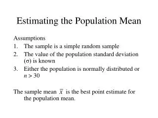
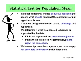
Statistical Test for Population Mean • In statistical testing, we use deductive reasoning to specify what should happen if the conjecture or null hypothesis is true. • A study is designed to collect data to challenge this hypothesis. • We determine if what we expected to happen is supported by the data. • If it is not supported, we reject the conjecture. • If it cannot be rejected we (tentatively) fail to reject the conjecture. • We have not proven the conjecture, we have simply not been able to disprove it with these data.
Logic Behind Statistical Tests Statistical tests are based on the concept of Proof by Contradiction. If P then Q=IfNOT Q then NOT P Analogy with justice system • Statistical Hypothesis Test • Start with null hypothesis, status quo. (Opposite is alternative hypothesis.) • If a significant amount of evidence is found to refute null hypothesis, reject it. (Enough evidence to conclude alternative is true.) • If not enough evidence found, we don’t reject the null. (Not enough evidence to disprove null.) • Court of Law • Start with premise that person is innocent. (Opposite is guilty.) • If enough evidence is found to show beyond reasonable doubt that person committed crime, reject premise. (Enough evidence that person is guilty.) • 3. If not enough evidence found, we don’t reject the premise. (Not enough evidence to conclude person guilty.)
Examples in Testing Logic CLAIM: A new variety of turf grass has been developed that is claimed to resist drought better than currently used varieties. CONJECTURE: The new variety resists drought no better than currently used varieties. DEDUCTION: If the new variety is no better than other varieties (P), then areas planted with the new variety should display the same number of surviving individuals (Q) after a fixed period without water than areas planted with other varieties. CONCLUSION: If more surviving individuals are observed for the new varieties than the other varieties (NOT Q), then we conclude the new variety is indeed not the same as the other varieties, but in fact is better (NOT P).
Five Parts of a Statistical Test Other HA: m< 530 m 530 H0: m≤ 530 HA: m > 530 1. Null Hypothesis (H0:) 2. Alternative Hypothesis (HA:) 3. Test Statistic (T.S.) Computed from sample data. Sampling distribution is known if the Null Hypothesis is true. 4. Rejection Region (R.R.) Reject H0 if the test statistic computed with the sample data is unlikely to come from the sampling distribution under the assumption that the Null Hypothesis is true. 5. Conclusion: Reject H0 or Do Not Reject H0 R.R. z* > za Or z* < -za Or|z*| > za/2
Hypotheses Research Hypotheses: The thing we are primarily interested in “proving”. Average height of the class Null Hypothesis: Things are what they say they are, status quo. (It’s common practice to always write H0 in this way, even though what is meant is the opposite of HA in each case.)
Test Statistic Some function of the data that uses estimates of the parameters we are interested in and whose sampling distribution is known when we assume the null hypothesis is true. Most good test statistics are constructed using some form of a sample mean. The Central Limit Theorem Of Statistics Why?
Developing a Test Statistic for the Population Mean Hypotheses of interest: Test Statistic: Sample Mean Under H0: the sample mean has a sampling distribution that is normal with mean 0. Under HA: the sample mean has a sampling distribution that is also normal but with a mean m1 that is different from m0.
Graphical View H0: True (3) (1) (2) HA1: True m1 m0 What would you conclude if the sample mean fell in location (1)? How about location (2)? Location (3)? Which is most likely 1, 2, or 3 when H0 is true?
Rejection Region H0: Assumed True Testing HA1: m > m0 Rejection Region m0 C1 Reject H0 if the sample mean is in the upper tail of the sampling distribution. How do we determine C1?
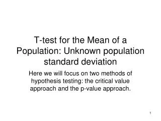
Determining the Critical Value for the Rejection Region Reject H0 if the sample mean is larger than “expected”. If H0 were true, we would expect 95% of sample means to be less than the upper limit of a 90% CI for μ. From the standard normal table. In this case, if we use this critical value, in 5 out of 100 repetitions of the study we would reject Ho incorrectly. That is, we would make an error. But, suppose HA1 is the true situation, then most sample means will be greater than C1 and we will be making the correct decision to reject more often.
Rejection Regions for Different Alternative Hypotheses 5% H0: m = m0 True Testing HA1: m > m0 Rejection Region C1 H0: m = m0 True Testing HA1: m < m0 5% Rejection Region C2 H0: m = m0 True Testing HA1: m m0 2.5% 2.5% Rejection Region C3L C3U m0
Type I Error If the sample mean is at location (1) or (3) we make the correct decision. a = P(Reject H0 when H0 is is the true condition) then a = 1/20=5/100 or .05 If If then the Type I error is a. H0: True Rejection Region m0 C1 (3) (2) (1) If the sample mean is at location (2) and H0 is actually true, we make the wrong decision. This is called making a TYPE I error, and the probability of making this error is usually denoted by the Greek letter a.
Type II Error If the sample mean is at location (1) or (3) we make the wrong decision. If the sample mean is at location (2) we make the correct decision. This is called making a TYPE II error, and the probability of making this type error is usually denoted by the Greek letter b. b = P(Do Not Reject H0 when HA is the true condition) We will come back to the Type II error later. HA1: True Rejection Region m1 m0 C1 (3) (2) (1)
Type I and II Errors Type I Error Region H0: True a Type II Error Region HA1: True b • We want to minimize the Type I error, just in case H0 is true, and we wish to minimize the Type II error just in case HA is true. • Problem: A decrease in one causes an increase in the other. • Also: We can never have a Type I or II error equal to zero! m1 m0 Rejection Region C1
Setting the Type I Error Rate The solution to our quandary is to set the Type I Error Rate to be small, and hope for a small Type II error also. The logic is as follows: 1. Assume the data come from a population with unknown distribution but which has mean (m) and standard deviation (s). 2. For any sample of size n from this population we can compute a sample mean, . 3. Sample means from repeated studies having samples of size n will have the sampling distribution of following a normal distribution with mean m and a standard deviation of s/n (the standard error of the mean). This is the Central Limit Theorem. 4. If the Null Hypothesis is true and m = m0, then we deduce that with probability a we will observe a sample mean greater than m0 + zas/n. (For example, for a = 0.05, za=1.645.)
Setting Rejection Regions for Given Type I Error Following this same logic, rejection rules for all three possible alternative hypotheses can be derived. Note: It is just easier to work with a test statistic that is standardized. We only need the standard normal table to find critical values. Reject Ho if: For (1-a)100% of repeated studies, if the true population mean is m0 as conjectured by H0, then the decision concluded from the statistical test will be correct. On the other hand, in a100% of studies, the wrong decision (a Type I error) will be made.
Risk a = 0.05 The value 0 < a < 1 represents the risk we are willing to take of making the wrong decision. But, what if I don’t wish to take any risk? Why not set a = 0? What if the true situation is expressed by the alternative hypothesis and not the null hypothesis? a = 0.01 a = 0.001 Suppose HA1 is really the true situation. Then the samples come from the distribution described by the alternative hypothesis and the sampling distribution of the mean will have mean m1, not m0. But this! m1 m0
The Rejection Rule (at an Type I error probability) or if 1 0 C1 Do not reject Ho Reject Ho Pretty clear cut when 1 much greater than 0
Error Probabilities When H0 is true 0 1 C1 When HA is true If HA is the true situation, then any sample whose mean is larger than will lead to the correct decision (reject H0, accept HA).
If HA is the true situation True Situation H0 : True HA : True Type I Error Correct 1 - Reject H0 Decision Correct 1 - Type II Error Accept H0 Then any sample such that its sample mean is less than will lead to the wrong decision (do not reject H0, reject HA). Do not reject HA Reject HA C1
Computing Error Probabilities Type I Error Probability (Reject H0 when H0 true) Power of the test. (Reject H0 when HA true) Type II Error Probability (Reject HA when HA true)
Example Sample Size: n = 50 Sample Mean: Sample Standard deviation: s = 5.6 H0: = 0 = 38 HA: > 38 What risk are we willing to take that we reject H0 when in fact H0 is true? P(Type I Error) = = .05 Critical Value: z.05 = 1.645 Rejection Region Conclusion: Reject H0
Type II Error. To compute the Type II error for a hypothesis test, we need to have a specific alternative hypothesis stated, rather than a vague alternative Vague HA: > 0 HA: < 0 HA: 0 Specific HA: = 1 > 0 HA: = 1<0 Note: As the difference between 0 and 1 getslarger, the probability of committing a Type II error (b) decreases. HA: = 5<10 HA: = 20>10 HA: m 10 Significant Difference: D = m0 - m1
Computing the probability of a Type II Error () H0: = 0 HA: = 1 > 0 0 H0: = 0 HA: = 1 < 0 1 H0: = 0 Ha: 0 = 1 0 0 1 1 - = Power of the test
Example: Power Assuming s is actually equal to s (usually what is done):
Power versus D (fixed n and s) Type II error As D gets larger, it is less likely that a Type II error will be made. 1-a b D
Power versus n(fixed D and s) Type II error As n gets larger, it is less likely that a Type II error will be made. 1-a b n What happens for larger s?
Power vs. Sample Size Power = 1-b D n b power 1 25 .857 .143 2 25 .565 .435 4 25 .054 .946 D n b power 1 50 .755 .245 2 50 .286 .714 4 50 .001 .999
Power Curve 1-a 1-a 0 0 0 0 large large D D n=50 Power 1-b n=10 See Table 4, Ott and Longnecker Pr(Type II Error) b
Summary 1) For fixed and n, decreases (power increases) as increases. 2) For fixed and , decreases (power increases) as n increases. 3) For fixed and n, decreases (power increases) as decreases.
Increasing Precision for fixed D increases Power N(m0,s/n) 1 < Decreasing decreases the spread in the sampling dist of Note: za changes. Same thing happens if you increase n. Same thing happens if is increased. N(m0,s1 /n)
Sample Size Determination • 1) Specify the critical difference, D (assume is known). • Choose P(Type I error) = and Pr(Type II error) = based on traditional and/or personal levels of risk. • One-sided tests: • Two-sided tests: Example: One-sided test, = 5.6, and we wish to show a difference of = .5 as significant (i.e. reject H0: = 0 for HA: = 1= 0 + ) with = .05 and = .2.