Understanding Stereo Coverage with Overlapping Aerial Photographs for 3D Measurements

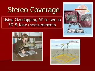
1. Stereo Coverage Using Overlapping AP to see in 3D & take measurements

2. Why use Stereo? • Can convey information • slopes, • shapes of landforms, • Elevations, • relationships between landforms & vegetation, • drainage systems

3. Determining Photo Orientation • Printed info/ annotation • Usually along N edge • (Sometimes E edge) • Cross-reference • map

4. Printed Info/Annotation • Date of Flight - always top left • Time - (optional) • f in mm (frequently 152.598 mm = 6”) • scale (RF) - (optional) • Roll #, Flight-line & Exposure # (always top right)

5. Flight-Line Overlap

6. Sidelap Flight lines are parallel Series of 3 along same flight line: stereotriplet

7. Stereo Pair

8. Drift & Crab Drift: lateral shift Crab: aircraft is not oriented with the flight-line

9. Stereo Viewing • Third dimension • Depth perception • Binocular or stereoscopic vision Parlor Stereoscope Creates the illusion of depth

10. Types of Stereoscopes • 1 – lens or pocket • Pair of magnifying lenses to keep lines of sight ~parallel • Relatively inexpensive • Narrow field of view – cannot see entire overlapped portion at once • 2 – mirror or reflecting • 3 – zoom

11. Types of Stereoscopes • 1 – lens or pocket • 2 – mirror or reflecting • Uses prisms & mirrors • Can provide full view • Widens viewer’s Eye Base • 3 – zoom

12. Types of Stereoscopes • 1 – lens or pocket • 2 – mirror or reflecting • 3 – zoom • Best technology • Variable magnification from 2X to 64X • Light table • Uncut photos

13. Stereo Viewing without instruments • Naked-eye stereoscopic viewing • Train your eyes to have parallel lines of sight • Practiced with “sausage link” exercise

14. Preparing AP for stereo viewing • Two overlapping AP • Flat surface • Trial & error basis • Move AP around under stereoscope • Use fingertips on same location on both photos • For precision work • Establish flight line

15. Orienting a Stereopair • adjacent overlapping photos • align them so that annotations are oriented along the left side of the AP 6-93 6-94

16. 6-93 6-94 Flight line Flight line PP CPP CPP PP Orienting a Stereopair • Locate the PP – draw lines between fiducial marks • Locate the conjugate principal point (CPP) • PP of the adjacent photo • Draw a line between the PP and CPP • flight line • Align the photos so that all 4 points lie on a straight line

18. Stereo Viewing • Overlap the photos • the separation distance between an object on one photo & its conjugate on the other photo • ~ equivalent to the eye base of the viewer (distance between pupils) • One lens - over one photo, • while the other lens is over the other photo • the long axis of the stereoscope aligned in parallel with the photo flight line

19. Principles of Photogrammetry The technique of obtaining reliable measurements of objects from AP -- Distance, area, height Accuracy of Scale - - essential

20. Map Scale things look large at large scale Large 1:24,000 1:500,000 1:3,000,000 Small things look small at small scale

21. Alternative ways to express Photographic Scale • 1:24,000 can be expressed as 1 in. = 2,000ft 12 inches in a foot - - 24,000/12 = 2,000ft 1:100,000 same as 1 cm = 1 km

22. 1 5.2 inches/5.2 inches 5.2 inches = = = 9748 50,688 inches 50,688 inches/5.2 inches D(m) 5.2 inches = D(g) .8 miles Scale Determination • 3 Methods • From Photo-Ground distance • RF= d(m)/d(g) • % of error minimized by measuring larger distances 1 mile = 63,360 inches, so 0.8 X 63360 = 50688 in

23. Objects of known measurements • Smaller objects = greater error

24. PD (MD)(MS) Scale Determination • From Photo-Map distances • Measurement on photo • Measurement on map of known scale RF = MD = map distance between 2 points MS = map-scale denominator PD = photo distance between same 2 points

25. PD (MD)(MS) RF = MD = map distance between 2 points MS = map-scale denominator PD = photo distance between same 2 points • Example PD = 3.2cm MD = 6 cm MS = 50,000 (Map RF=1:50,000) RF = 3.2 cm = 3.2 cm = 1 6 cm * 50,000 300,000 cm 93,750 RF = 1:93,750

26. Scale - - Photo-Map distances • 2 points selected: • Diametrically opposed • A line connecting them passes through or near the PP • Points are ~equidistant from PP • Distortion minimized • Preferred: points be at same or similar elevation

27. Scale Determination • From Focal Length & Altitude • RF= f/H • Principles of geometry • Determining relationship between film plane & terrain • f= focal length • H= height above terrain (mean) from which exposure was made

28. f DE = H AB PP D E Film Plane f C Lens <ACB = <DC E Relationship between Similar triangles H Terrain A B Nadir

29. Average Scale Example: f = 210 mm H = 2,500 m MSL & ground elevation = 400 m RF = 210 mm * 1m = 210 . (2,500 m - 400 m) 1000 mm 2,100,000 (2,100m) RF = 1 or 1:10,000 10,000 Precise only if landscape is uniformly 400m above MSL

30. Scale varies directly with f and inversely with flying height (H) • As f increases, scale increases (“zooming in”) • (larger scale - - covers smaller area) • As flying height increases, scale decreases (smaller scale - - covers larger area) long focal length lens - - requires more photos to cover a given land area (assuming constant H)

32. f DE = H AB PP D E Film Plane f increases scale increases - More detail - f C Lens H increases, scale decreases - Less detail - H Terrain A B Nadir

33. RF = f/H Example: f = 210 mm H = 2,500 m MSL & ground elevation = 400 m RF = 210 mm * 1m = 210 . = 210/210 = 1:10,000 (2,500 m - 400 m) 1000 mm 2,100,000 2,100,00/210 (2,100m) Increase H to 4,000 m MSL (same ground elevation = 400m) RF = 210 mm * 1m = 210 . = 1: 17,142 (4,000 m – 400m) 1000mm 3,600,000 Smaller scale Less detail Increase the number on bottom of fraction: Smaller scale Increase the number on top of fraction: Larger Scale

34. Same focal length/lens angle • Plane A: • smaller scale, • less detail, • fewer photos A A = 1:100,000 B B = 1:10,000 H H’

35. 3 Photo Centers: Principal Point, Nadir, Isocenter • Principal Point • point where the perpendicular projected through the center of the lens intersects the photo image • Nadir: • point vertically beneath the camera center at the time of exposure • Isocenter • point on the photo that falls on a line half- way between the principal point & the Nadir point

36. Principal Point (PP) • Geometric center of photograph (center of lens) PP Fiducial Marks Nadir = point on the ground that coincides with PP (on true vertical photo)

37. Displacement

38. Tilt Displacement • Slightly oblique (2-3 degrees or less can be ignored)

39. Relief Displacement • As objects vary in height, the camera sees the sides • Objects appear to lean – outward from PP • The greater the height, the greater the displacement • The farther the object from the PP, the greater the displacement

40. Tank B shows more displacement because it is farther from the nadir • ~same height • Can measure if nadir & PP are same position

42. Aerial Photography: Applications Land Use/Cover Change Detection

43. Land Cover & Land Use • LC: the biophysical material covering the earth’s surface • LU: how humans are using the land surface • LC : impervious surface • LU : parking lot • LC : grass • LU : recreational field

44. LU/LC Classification Systems • Systematic categorization of LU or LC types • Often hierarchical, progressing from the general to the specific, • e.g., level I --> level II --> level III 1 Urban or built-up 2 Agricultural land 3 Grass/Rangeland 4 Forest land 5 Water 6 Wetland 7 Barren land 8 Tundra 9 Perennial snow or ice Example: USGS LU/LC

46. 1 Urban or built-up land Components of Suburban development: houses, roads, lawns, sidewalks “Brownfield”, Camden, NJ

47. 2 Agricultural land Agricultural landscape Associated buildings: barns, silos 21 Crop land: from planting to harvest

48. 2 Agricultural land 22 Nursery: trees 24 Other: cranberry bog

49. 3 Grass/Rangeland 32 Shrub and brush rangeland Tierra del Fuego, Chile 31 Herbaceous grass/rangeland Konza Prairie, Kansas

50. 4 Forest 42 Evergreen: Conifer Sierras, CA 41 Deciduous - New Forest, UK 42 Evergreen: broadleaved Costa Rica 43 Mixed - Pine Barrens, NJ