Frequency Response Bode plots Examples
Lecture 22. Bode Plots. Frequency Response Bode plots Examples. Frequency Response. The transfer function can be separated into magnitude and phase angle information H (j ) = | H (j ) | Φ (j ). e.g., . H (j )= Z (j w ) . Bode Plots.

Frequency Response Bode plots Examples
E N D
Presentation Transcript
Lecture 22. Bode Plots • Frequency Response • Bode plots • Examples
Frequency Response • The transfer function can be separated into magnitude and phase angle information H(j) = |H(j)| Φ(j) e.g., H(j)=Z(jw)
Bode Plots • A Bode plot is a (semilog) plot of the transfer function magnitude and phase angle as a function of frequency • The gain magnitude is many times expressed in terms of decibels (dB) dB = 20 log10 A where A is the amplitude or gain • a decade is defined as any 10-to-1 frequency range • an octave is any 2-to-1 frequency range 20 dB/decade = 6 dB/octave
Bode Plots • Straight-line approximations of the Bode plot may be drawn quickly from knowing the poles and zeros • response approaches a minimum near the zeros • response approaches a maximum near the poles • The overall effect of constant, zero and pole terms
Bode Plots • Express the transfer function in standard form • There are four different factors: • Constant gain term, K • Poles or zeros at the origin, (j)±N • Poles or zeros of the form (1+ j) • Quadratic poles or zeros of the form 1+2(j)+(j)2
Bode Plots • We can combine the constant gain term (K) and the N pole(s) or zero(s) at the origin such that the magnitude crosses 0 dB at • Define the break frequency to be at ω=1/ with magnitude at ±3 dB and phase at ±45°
Bode Plot Summary where N is the number of roots of value τ
Single Pole & Zero Bode Plots ωp Gain ωz Gain +20 dB 0 dB 0 dB –20 dB ω ω One Decade Phase Phase One Decade +90° 0° +45° –45° 0° –90° ω ω Zero at ωz=1/ Pole at ωp=1/ Assume K=1 20 log10(K) = 0 dB
Bode Plot Refinements • Further refinement of the magnitude characteristic for first order poles and zeros is possible since Magnitude at half break frequency: |H(½b)| = ±1 dB Magnitude at break frequency: |H(b)| = ±3 dB Magnitude at twice break frequency: |H(2b)| = ±7 dB • Second order poles (and zeros) require that the damping ratio ( value) be taken into account; see Fig. 9-30 in textbook
Bode Plots to Transfer Function • We can also take the Bode plot and extract the transfer function from it (although in reality there will be error associated with our extracting information from the graph) • First, determine the constant gain factor, K • Next, move from lowest to highest frequency noting the appearance and order of the poles and zeros
|H(ω)| +20 dB/decade –20 dB/decade 6 dB –40 dB/decade ω (rad/sec) 0.1 0.7 2 11 90 Class Examples • Drill Problems P9-3, P9-4, P9-5, P9-6 (hand-drawn Bode plots) • Determine the system transfer function, given the Bode magnitude plot below
Class Examples • Drill Problems P9-3, P9-4, P9-5