SIFT paper
SIFT paper. Terms & Definitions. Pose = position + orientation of an object Image gradient = change in brightness (orientation dependent) Scale = ‘size’ of features. Gaussian filters eliminate ‘smaller’ features

SIFT paper
E N D
Presentation Transcript
Terms & Definitions • Pose = position + orientation of an object • Image gradient = change in brightness (orientation dependent) • Scale = ‘size’ of features. Gaussian filters eliminate ‘smaller’ features • Octave = a set of scales that goes up to a double, e.g. 1, sqrt(2), 2 is an octave.
Overview • Scale space extrema detection • Potential image points from DoG function, invariant to scale and orientation • Keypoint localization • Choose stable locations & determine their exact position & scale • Orientation assignment • Assign keypoint orientation based on image gradients • Keypoint Descriptor = final representation
Using the SIFT • Collect keypoints for each reference image and store in database • Collect keypoints for the ‘unknown’ image • Look for clusters of matches • Agree on object, scale, and image location • Compute probability of object, given features
Related Research • Corner & feature detectors (Moravec, Harris) • Feature matching into database (Schmid & Mohr) • Feature scale invariance (Lowe) • Affine invariant matching (many) • Alternative feature types (many)
Detection of Scale Space Extrema • Scale space: (x, y, sigma) • Sigma is parameter of a Gaussian function • Extrema in scale space • Pixel whose values is max (min) of local window • Difference of Gaussian function • D(x,y,sigma) = (G(x, y, k*sigma) – G(x, y, sigma)) * I(x,y) • first create DoG kernel, then convolve with image
Difference of Gaussian http://fourier.eng.hmc.edu/e161/lectures/gradient/node11.html
Local Extrema Detection Szeliski: Fig 4.11
How many scales? • In Section 3.2, experiments show: • Repeatability peaks at 3 scales / octave, then slowly drops off • Number of keypoints grows as scales grow, but slowly than linear (appears approx. log) • Bottom line: they chose 3 scales / octave
Keypoint localization • Initial implementation: location/scale of keypoint taken from pixel coordinates in scale space • Improved implementation: • Fit 3D quadratic function to local sample points • Return coordinates of peak of fit function (subpixel) – see equations 2 and 3 • If value of D(x, y, sigma) is too small, reject due to low contrast
Avoiding Edges • A point on an edge does not localize well (it can slide along the edge) • Compute Dxx, Dxy, Dyy (as we did last week) • Tr(H) = Dxx + Dyy • Det(H) = DxxDyy – Dxy*Dxy • If (Tr(H)*Tr(H))/Det(H) > 12.1 (using r of 10), then location is eliminated (max curvature / min curvature > 10)
Keypoint Orientation • Depends on local image properties (e.g. intensities) • Choose the Gaussian smoothed image L at the keypoint’s scale • Compute gradients using horizontal and vertical [1 0 -1] masks (call them H and V) • Gradient magnitude = sqrt(H*H+V*V) • Gradient direction = atan(V/H)
Orientation Histogram • Collect orientations in window around sample point • Weights fall off based on Gaussian with sigma that is 1.5 times scale • Build histogram (36 bins) of weighted orientations • Peak of histogram is keypoint orientation • Any other peaks within 80% are additional keypoint orientations
Local image descriptor • Each keypoint has image location, scale, and orientation • Descriptor is array of histograms of orientations surrounding the keypoint (See Fig. 7) • Array is normalized to reduce effects of lighting
Application: Object Recognition • Match each keypoint independently to database (nearest neighbor) • Find clusters of at least 3 features that agree on object, position and orientation (pose) • Perform detailed geometric fit to model and accept or reject